Introduction
An essential part of any data analysis project is to understand the data at hand. For this task, we will create a function that takes as input a variable from the data, a categorical variable to describe by, and returns summary tables and plots.
This presentation uses the R programming language and assumes the end user is taking advantage of RStudio IDE to compile their R markdown files into HTML (R Core Team 2019; RStudio Team 2016). All of the files needed to reproduce these results can be downloaded from the Git repository git clone https://git.waderstats.com/data_summaries/.
Required Libraries
The libraries knitr, bookdown, and kableExtra are used to generate the HTML output (Xie 2019, 2018; Zhu 2019). The ggplot2 library is loaded for the example data set that is used in this presentation (Wickham 2016). The Hmisc library provides functionality needed to create variable labels (Harrell Jr, Charles Dupont, and others. 2019). The libraries reshape2 and dplyr are loaded for their data manipulation funtions (Wickham et al. 2019; Wickham 2007).
package_loader <- function(x, ...) {
  if (x %in% rownames(installed.packages()) == FALSE) install.packages(x)
  library(x, ...)
}

packages <- c("knitr", "bookdown", "kableExtra", "ggplot2", "Hmisc", "reshape2", "dplyr")

invisible(sapply(X = packages, FUN = package_loader, character.only = TRUE))
Example Data Setup
The data set used in this presentation is mpg from the ggplot2 package. From the description in the manual:
This dataset contains a subset of the fuel economy data that the EPA makes available here. It contains only models which had a new release every year between 1999 and 2008 - this was used as a proxy for the popularity of the car.
set.seed(123)
data(mpg)
mpg <- data.frame(mpg)

colnames(mpg)[which(colnames(mpg) == "manufacturer")] <- "manu"

mpg$manu <- factor(mpg$manu)
mpg$model <- factor(mpg$model)
mpg$displ <- as.numeric(mpg$displ)
mpg$year <- factor(mpg$year, levels = c("1999", "2008"), ordered = TRUE)

mpg$dp <- as.Date(NA, origin = "1970-01-01")
mpg$dp[which(mpg$year == "1999")] <- sample(seq(as.Date('1999-01-01', format = "%Y-%m-%d", origin = "1970-01-01"), as.Date('1999-12-25', format = "%Y-%m-%d", origin = "1970-01-01"), by="day"), dim(mpg)[1]/2)
mpg$dp[which(mpg$year == "2008")] <- sample(seq(as.Date('2008-01-01', format = "%Y-%m-%d", origin = "1970-01-01"), as.Date('2008-12-25', format = "%Y-%m-%d", origin = "1970-01-01"), by="day"), dim(mpg)[1]/2)
mpg$dp[sample(1:length(mpg$dp), size = 20)] <- NA
mpg$dp[10] <- as.Date('1000-05-02', format = "%Y-%m-%d", origin = "1970-01-01")

mpg$dplt <- as.POSIXlt(NA, origin = "1970-01-01 0:0:0")
mpg$dplt[which(mpg$year == "1999")] <- sample(seq(as.POSIXlt('1999-01-01 0:0:0', format = "%Y-%m-%d %H:%M:%S", origin = "1970-01-01 0:0:0"), as.POSIXlt('1999-12-25 0:0:0', format = "%Y-%m-%d %H:%M:%S", origin = "1970-01-01 0:0:0"), by="min"), dim(mpg)[1]/2)
mpg$dplt[which(mpg$year == "2008")] <- sample(seq(as.POSIXlt('2008-01-01 0:0:0', format = "%Y-%m-%d %H:%M:%S", origin = "1970-01-01 0:0:0"), as.POSIXlt('2008-12-25 0:0:0', format = "%Y-%m-%d %H:%M:%S", origin = "1970-01-01 0:0:0"), by="sec"), dim(mpg)[1]/2)
mpg$dplt[sample(1:length(mpg$dplt), size = 20)] <- NA

mpg$dpct <- as.POSIXct(NA, origin = "1970-01-01 0:0:0")
mpg$dpct[which(mpg$year == "1999")] <- sample(seq(as.POSIXct('1999-01-01 0:0:0', format = "%Y-%m-%d %H:%M:%S", origin = "1970-01-01 0:0:0"), as.POSIXct('1999-12-25 0:0:0', format = "%Y-%m-%d %H:%M:%S", origin = "1970-01-01 0:0:0"), by="min"), dim(mpg)[1]/2)
mpg$dpct[which(mpg$year == "2008")] <- sample(seq(as.POSIXct('2008-01-01 0:0:0', format = "%Y-%m-%d %H:%M:%S", origin = "1970-01-01 0:0:0"), as.POSIXct('2008-12-25 0:0:0', format = "%Y-%m-%d %H:%M:%S", origin = "1970-01-01 0:0:0"), by="sec"), dim(mpg)[1]/2)
mpg$dpct[sample(1:length(mpg$dpct), size = 20)] <- NA

mpg$cyl <- factor(mpg$cyl, levels = c(4, 5, 6, 8), ordered = TRUE)

mpg$trans <- factor(mpg$trans)
mpg$drv <- factor(mpg$drv, levels = c("f", "r", "4"), labels = c("front-wheel drive", "rear wheel drive", "4wd"))
mpg$fl <- factor(mpg$fl)
mpg$class <- factor(mpg$class)

mpg$rn <- rnorm(dim(mpg)[1], mean = 10, sd = 5)
mpg$rn[sample(1:length(mpg$rn), size = 50)] <- NA

mpg$rdifftime <- rnorm(dim(mpg)[1], mean = 10, sd = 5)
mpg$rdifftime[sample(1:length(mpg$rdifftime), size = 50)] <- NA
mpg$rdifftime <- as.difftime(mpg$rdifftime, units = "weeks")
mpg$rdifftime[which(mpg$rdifftime < 0)] <- 0

mpg$logical <- mpg$rdifftime >= 10

mpg$party <- factor(sample(c("republican", "democrat", "independent", NA), dim(mpg)[1], replace = TRUE), levels = c("republican", "democrat", "independent"))

mpg$comments <- sample(c("I like this car!", "Meh.", "This is the worst car ever!", "Does it come in green?", "want cheese flavoured cars.", "Does it also fly?", "Blah, Blah, Blah, Blah, Blah, Blah, Blah, Blah", "Missing", ".", NA), dim(mpg)[1], replace = TRUE)

mpg$miss <- NA

label(mpg$manu) <- "manufacturer"
label(mpg$model) <- "model name"
label(mpg$displ) <- "engine displacement, in litres"
label(mpg$year) <- "year of manufacture"
label(mpg$dp) <- "date of purchase (Date class)"
label(mpg$dplt) <- "date of purchase (POSIXlt class)"
label(mpg$dpct) <- "date of purchase (POSIXct class)"
label(mpg$cyl) <- "number of cylinders"
label(mpg$trans) <- "type of transmission"
label(mpg$drv) <- "drive type"
label(mpg$cty) <- "city miles per gallon"
label(mpg$hwy) <- "highway miles per gallon"
label(mpg$fl) <- "fuel type"
label(mpg$class) <- "type of car"
label(mpg$rn) <- "some random numbers that are generated from a normal distrubtion with mean = 10 and sd = 5"
label(mpg$rdifftime) <- "some random numbers that are generated from a normal distrubtion with mean = 10 and sd = 5, and then converted to weeks"
label(mpg$logical) <- "some random numbers that are generated from a normal distrubtion with mean = 10 and sd = 5, and then converted to weeks, and then set to TRUE if the difference is greater than 10"
label(mpg$party) <- "some random political parties"
label(mpg$comments) <- "some random comments"
label(mpg$miss) <- "an all missing variable"

kable(head(mpg), caption = "Header of <b>mpg</b>.", booktabs = TRUE, escape = FALSE) %>% kable_styling(bootstrap_options = c("striped", "hover", "condensed", "responsive"))| manu | model | displ | year | cyl | trans | drv | cty | hwy | fl | class | dp | dplt | dpct | rn | rdifftime | logical | party | comments | miss |
|---|---|---|---|---|---|---|---|---|---|---|---|---|---|---|---|---|---|---|---|
| audi | a4 | 1.8 | 1999 | 4 | auto(l5) | front-wheel drive | 18 | 29 | p | compact | 1999-06-28 | 1999-10-07 07:18:00 | 1999-10-27 07:00:00 | 8.935759 | 9.675375 weeks | FALSE | NA | Blah, Blah, Blah, Blah, Blah, Blah, Blah, Blah | NA |
| audi | a4 | 1.8 | 1999 | 4 | manual(m5) | front-wheel drive | 21 | 29 | p | compact | 1999-01-14 | 1999-04-28 06:00:00 | 1999-01-25 04:26:00 | 9.531816 | 13.782912 weeks | TRUE | democrat | Does it also fly? | NA |
| audi | a4 | 2.0 | 2008 | 4 | manual(m6) | front-wheel drive | 20 | 31 | p | compact | 2008-02-08 | 2008-05-04 13:32:00 | 2008-01-06 09:57:35 | 9.566429 | 4.928852 weeks | FALSE | independent | . | NA |
| audi | a4 | 2.0 | 2008 | 4 | auto(av) | front-wheel drive | 21 | 30 | p | compact | 2008-07-14 | 2008-02-11 12:43:49 | 2008-01-30 06:40:31 | 17.207309 | 6.539646 weeks | FALSE | democrat | Does it come in green? | NA |
| audi | a4 | 2.8 | 1999 | 6 | auto(l5) | front-wheel drive | 16 | 26 | p | compact | 1999-07-14 | 1999-07-22 12:22:00 | 1999-03-02 01:18:00 | NA | NA weeks | NA | NA | . | NA |
| audi | a4 | 2.8 | 1999 | 6 | manual(m5) | front-wheel drive | 18 | 26 | p | compact | 1999-11-02 | 1999-08-20 07:26:00 | 1999-04-03 22:19:00 | 14.172008 | 8.202642 weeks | FALSE | NA | This is the worst car ever! | NA |
Data Summary Function
Below are a set of functions I wrote to using S4 (see https://www.cyclismo.org/tutorial/R/s4Classes.html for a gentle introduction to object oriented programming in R), culminating into a single function called data_summary. The basic structure uses an object of class dataSummaries and then, based on the class of x, the dataSummariesSetup method applied to the dataSummaries class, returns an object of class dataSummariesCharacter, dataSummariesNumeric, dataSummariesDate, or dataSummariesDifftime. Each of these four output classes inherits from the dataSummaries class; thus any method written for dataSummaries also applies to the four classes that inherit from it.
As input the data_summary function takes a variable to summarize (x), an optional variable or variables (as a character string) to summarize by (by), the data (data), and the units to use for difftime if x refers to a Date, POSIXlt, POSIXct, or difftime object in the data.
As output, the function returns an object of class dataSummaries. The function has a show method and a method called make_output that generates knitr friendly output. The summary table and plot can also be accessed individually through their accessor functions, data_summary_table, and data_summary_plot, respectively.
If you find any bugs or have recommendations, let me know in the comments!
setOldClass(c("gg", "ggplot"))
dataSummaries <- setClass(
"dataSummaries",
slots = c(
x = "character",
by = "character",
data = "data.frame",
difftime_units = "character",
xLab = "character",
byLab = "character",
table = "data.frame",
plot = "ggplot"
),
prototype = list(
x = character(0),
by = character(0),
data = data.frame(),
difftime_units = character(0),
xLab = character(0),
byLab = character(0),
table = data.frame(),
plot = ggplot()
)
)
dataSummariesCharacter <- setClass(
"dataSummariesCharacter",
slots = c(
type = "character"
),
prototype = list(
type = character(0)
),
contains = "dataSummaries"
)
dataSummariesNumeric <- setClass(
"dataSummariesNumeric",
slots = c(
type = "character"
),
prototype = list(
type = character(0)
),
contains = "dataSummaries"
)
dataSummariesDate <- setClass(
"dataSummariesDate",
slots = c(
type = "character"
),
prototype = list(
type = character(0)
),
contains = "dataSummaries"
)
dataSummariesDifftime <- setClass(
"dataSummariesDifftime",
slots = c(
type = "character"
),
prototype = list(
type = character(0)
),
contains = "dataSummaries"
)
invisible(setGeneric(name = "dataSummariesSetup", def = function(object) standardGeneric("dataSummariesSetup")))
setMethod(f = "dataSummariesSetup",
signature = "dataSummaries",
definition = function(object)
{
x = object@x
by = object@by
data = object@data
xLab <- label(data[, x])
colnames(data)[which(colnames(data) == x)] <- "var"
if (length(by) == 0) {
data$by <- factor(data$by <- "")
label(data$by) <- ""
byLab <- label(data$by)
} else {
data$by <- interaction(data[, by], sep = ", ")
byLab <- paste(label(data[, by]), collapse = " by ")
overall <- data
overall$by <- "Overall"
data <- rbind(data, overall)
}
data <- data[, c("var", "by")]
if("labelled" %in% class(data$var)) {
class(data$var) <- class(data$var)[(-1)*which(class(data$var) == "labelled")]
}
object@xLab <- xLab
object@byLab <- byLab
object@data <- data
if (any(c("character", "factor", "logical") %in% class(data$var))) {
return(dataSummariesCharacter(object, type = class(data$var)))
} else if (any(c("numeric", "integer") %in% class(data$var))) {
return(dataSummariesNumeric(object, type = class(data$var)))
} else if (any(c("Date", "POSIXlt", "POSIXct", "POSIXt") %in% class(data$var))) {
if (length(object@difftime_units) == 0) stop("You need to specify the units for the difference in time. See help(difftime) for additional information.")
return(dataSummariesDate(object, type = class(data$var)))
} else if ("difftime" %in% class(data$var)) {
if (length(object@difftime_units) == 0) stop("You need to specify the units for the difference in time. See help(difftime) for additional information.")
return(dataSummariesDifftime(object, type = class(data$var)))
} else {
stop("x is an unsupported class")
}
}
)
invisible(setGeneric(name = "data_summary_switch", def = function(object) standardGeneric("data_summary_switch")))
setMethod(f = "data_summary_switch",
signature = "dataSummariesCharacter",
definition = function(object)
{
xLab <- object@xLab
byLab <- object@byLab
data <- object@data
freqs <- table(data$var, data$by, useNA = "ifany", dnn = c(xLab, byLab))
rownames(freqs)[which(is.na(rownames(freqs)))] <- "R NA Value"
colnames(freqs)[which(is.na(colnames(freqs)))] <- "R NA Value"
props <- round(100*prop.table(freqs, 2), 2)
res <- freqs
for (i in 1:dim(freqs)[2]) {
res[, i] <- paste(freqs[, i], " (", props[, i], "%)", sep = "")
}
res <- as.data.frame(res)
colnames(res) <- c("var", "by", "freq")
res <- dcast(res, var ~ by, value.var = "freq")
colnames(res)[1] <- xLab
if (byLab == "") colnames(res)[2] <- "n (%)"
pData <- as.data.frame(props)
colnames(pData) <- c("var", "by", "freq")
levs <- as.character(pData$var)
tmp <- nchar(levs)
strCombRes <- list()
for (k in 1:length(levs)) {
strRes <- list()
j = 0
for (i in 1:ceiling(max(tmp)/30)) {
strRes[[i]] <- substr(levs[k], j, 30*i)
j = 30*i + 1
}
strCombRes[[k]] <- unlist(strRes)
}
foo <- function(x) {
if (!(length(which(x == "")) == 0)) x <- x[-1*which(x == "")]
x <- paste(x, collapse = "\n")
return(x)
}
levs <- unlist(lapply(strCombRes, foo))
pData$names <- factor(rownames(pData), levels = rownames(pData), labels = levs)
pData <- pData[, -1]
colfunc <- colorRampPalette(c("#e41a1c","#377eb8","#4daf4a","#984ea3","#ff7f00"))
colors <- colfunc(length(levels(pData$names)))
p = ggplot(data = pData, aes(x = by, y = freq, fill = names)) +
scale_fill_manual(values = colors) +
geom_bar(stat = "identity") +
xlab(paste(strwrap(xLab, width = 60), collapse = "\n")) +
ylab("Percent") +
theme(axis.line = element_line(colour = "black"),
panel.border = element_rect(colour = "black", fill = NA, size = 1),
axis.text = element_text(size = 12),
axis.text.x = element_text(angle = 50, hjust = 1),
axis.title = element_text(size = 12),
legend.title = element_blank(),
legend.position = "right",
panel.grid = element_line(color = "lightgray"),
panel.background = element_rect(fill = "white", colour = "white"))
object@table <- res
object@plot <- p
return(object)
}
)
setMethod(f = "data_summary_switch",
signature = "dataSummariesNumeric",
definition = function(object)
{
xLab <- object@xLab
byLab <- object@byLab
data <- object@data
if (any(is.na(data$by))) {
byLevs <- levels(data$by)
data$by <- as.character(data$by)
data$by[which(is.na(as.character(data$by)))] <- "R NA Value"
data$by <- factor(data$by, levels = c(byLevs, "R NA Value"))
}
percMiss <- function(x) res <- round((length(which(is.na(x)))/length(x))*100, 2)
res <- data %>%
group_by(by) %>%
summarize(label = xLab,
n = length(na.omit(var)),
miss = percMiss(var),
mean = round(mean(var, na.rm = TRUE), 2),
sd = round(sd(var, na.rm = TRUE), 2),
median = round(median(var, na.rm = TRUE), 2),
mad = round(mad(var, na.rm = TRUE), 2),
q25 = round(quantile(var, probs = 0.25, na.rm = TRUE, type = 1), 2),
q75 = round(quantile(var, probs = 0.75, na.rm = TRUE, type = 1), 2),
IQR = round(IQR(var, na.rm = TRUE), 2),
min = round(min(var, na.rm = TRUE), 2),
max = round(max(var, na.rm = TRUE), 2)
)
res <- data.frame(res)
colnames(res) <- c(byLab, "Label", "N", "P NA", "Mean", "S Dev", "Med", "MAD", "25th P", "75th P", "IQR", "Min", "Max")
pData <- na.omit(data.frame(data[, c("var", "by")]))
p = ggplot(data = pData, aes(x = by, y = var)) +
geom_boxplot(position = position_dodge(1), fill = "#2c7bb6") +
xlab(byLab) +
ylab(paste(strwrap(xLab, width = 40), collapse = "\n")) +
theme(axis.line = element_line(colour = "black"),
panel.border = element_rect(colour = "black", fill = NA, size = 1),
legend.position = "none",
axis.text = element_text(size = 12),
axis.text.x = element_text(angle = 50, hjust = 1),
axis.title = element_text(size = 12),
panel.grid = element_line(color = "lightgray"),
panel.background = element_rect(fill = "white", colour = "white"))
object@table <- res
object@plot <- p
return(object)
}
)
setMethod(f = "data_summary_switch",
signature = "dataSummariesDate",
definition = function(object)
{
xLab <- object@xLab
byLab <- object@byLab
data <- object@data
difftime_units <- object@difftime_units
if (any(is.na(data$by))) {
byLevs <- levels(data$by)
data$by <- as.character(data$by)
data$by[which(is.na(as.character(data$by)))] <- "R NA Value"
data$by <- factor(data$by, levels = c(byLevs, "R NA Value"))
}
percMiss <- function(x) round((length(which(is.na(x)))/length(x))*100, 2)
sdDate <- function(x) {
res <- difftime(x, mean(x, na.rm = TRUE), units = "secs")
res <- as.numeric(as.character(res))
res <- sd(res, na.rm = TRUE)
res <- as.difftime(res, units = "secs")
units(res) <- difftime_units
return(res)
}
sdDate(data$var)
madDate <- function(x) {
res <- difftime(x, mean(x, na.rm = TRUE), units = "secs")
res <- as.numeric(as.character(res))
res <- mad(res, na.rm = TRUE)
res <- as.difftime(res, units = "secs")
units(res) <- difftime_units
return(res)
}
dquantile <- function(x, probs){
sx <- sort(x)
pos <- round(probs*length(x))
return(sx[pos])
}
q25Date <- function(x) dquantile(x, probs = 0.25)
q75Date <- function(x) dquantile(x, probs = 0.75)
IQRdate <- function(x) {
res <- difftime(dquantile(x, probs = 0.75), dquantile(x, probs = 0.25), units = "secs")
units(res) <- difftime_units
return(res)
}
res <- data %>%
group_by(by) %>%
summarize(label = xLab,
n = length(na.omit(var)),
miss = percMiss(var),
mean = mean(var, na.rm = TRUE),
sd = round(sdDate(var), 2),
median = median(var, na.rm = TRUE),
mad = round(madDate(var), 2),
q25 = q25Date(var),
q75 = q75Date(var),
IQR = IQRdate(var),
min = min(var, na.rm = TRUE),
max = max(var, na.rm = TRUE)
)
res <- data.frame(res)
colnames(res) <- c(byLab, "Label", "N", "P NA", "Mean", "S Dev", "Med", "MAD", "25th P", "75th P", "IQR", "Min", "Max")
pData <- na.omit(data.frame(data[, c("var", "by")]))
if("POSIXlt" %in% class(pData$var)) pData$var <- as.POSIXct(pData$var)
p = ggplot(data = pData, aes(x = by, y = var)) +
geom_boxplot(position = position_dodge(1), fill = "#2c7bb6") +
xlab(byLab) +
ylab(paste(strwrap(xLab, width = 40), collapse = "\n")) +
theme(axis.line = element_line(colour = "black"),
panel.border = element_rect(colour = "black", fill = NA, size = 1),
legend.position = "none",
axis.text = element_text(size = 12),
axis.text.x = element_text(angle = 50, hjust = 1),
axis.title = element_text(size = 12),
panel.grid = element_line(color = "lightgray"),
panel.background = element_rect(fill = "white", colour = "white"))
object@table <- res
object@plot <- p
return(object)
}
)
setMethod(f = "data_summary_switch",
signature = "dataSummariesDifftime",
definition = function(object)
{
xLab <- object@xLab
byLab <- object@byLab
data <- object@data
difftime_units <- object@difftime_units
if (any(is.na(data$by))) {
byLevs <- levels(data$by)
data$by <- as.character(data$by)
data$by[which(is.na(as.character(data$by)))] <- "R NA Value"
data$by <- factor(data$by, levels = c(byLevs, "R NA Value"))
}
percMiss <- function(x) res <- round((length(which(is.na(x)))/length(x))*100, 2)
units(data$var) <- "days"
meanDate <- function(x) {
res <- mean(x, na.rm = TRUE)
units(res) <- difftime_units
return(res)
}
medianDate <- function(x) {
res <- median(x, na.rm = TRUE)
units(res) <- difftime_units
return(res)
}
sdDate <- function(x) {
res <- as.difftime(sd(as.numeric(x), na.rm = TRUE), format = "%X", units = "days")
units(res) <- difftime_units
return(res)
}
madDate <- function(x) {
res <- as.difftime(mad(as.numeric(x), na.rm = TRUE), format = "%X", units = "days")
units(res) <- difftime_units
return(res)
}
q25Date <- function(x) {
res <- as.difftime(quantile(as.numeric(x), probs = 0.25, na.rm = TRUE, type = 1), units = "days")
units(res) <- difftime_units
return(res)
}
q75Date <- function(x) {
res <- as.difftime(quantile(as.numeric(x), probs = 0.75, na.rm = TRUE, type = 1), units = "days")
units(res) <- difftime_units
return(res)
}
IQRdate <- function(x) {
res <- as.difftime(IQR(as.numeric(x), na.rm = TRUE), format = "%X", units = "days")
units(res) <- difftime_units
return(res)
}
minDate <- function(x) {
res <- as.difftime(min(as.numeric(x), na.rm = TRUE), format = "%X", units = "days")
units(res) <- difftime_units
return(res)
}
maxDate <- function(x) {
res <- as.difftime(max(as.numeric(x), na.rm = TRUE), format = "%X", units = "days")
units(res) <- difftime_units
return(res)
}
res <- data %>%
group_by(by) %>%
summarize(label = xLab,
n = length(na.omit(var)),
miss = percMiss(var),
mean = round(meanDate(var), 2),
sd = round(sdDate(var), 2),
median = round(medianDate(var), 2),
mad = round(madDate(var), 2),
q25 = round(q25Date(var), 2),
q75 = round(q75Date(var), 2),
IQR = round(IQRdate(var), 2),
min = round(minDate(var), 2),
max = round(maxDate(var), 2)
)
res <- data.frame(res)
colnames(res) <- c(byLab, "Label", "N", "P NA", "Mean", "S Dev", "Med", "MAD", "25th P", "75th P", "IQR", "Min", "Max")
pData <- na.omit(data.frame(data[, c("var", "by")]))
units(pData$var) <- difftime_units
p = ggplot(data = pData, aes(x = by, y = var)) +
geom_boxplot(position = position_dodge(1), fill = "#2c7bb6") +
xlab(byLab) +
ylab(paste(strwrap(xLab, width = 40), collapse = "\n")) +
theme(axis.line = element_line(colour = "black"),
panel.border = element_rect(colour = "black", fill = NA, size = 1),
legend.position = "none",
axis.text = element_text(size = 12),
axis.text.x = element_text(angle = 50, hjust = 1),
axis.title = element_text(size = 12),
panel.grid = element_line(color = "lightgray"),
panel.background = element_rect(fill = "white", colour = "white"))
object@table <- res
object@plot <- p
return(object)
}
)
setMethod(f = "show",
signature = "dataSummaries",
definition = function(object)
{
print(object@table)
print(object@plot)
}
)
invisible(setGeneric(name = "make_kable_output", def = function(object) standardGeneric("make_kable_output")))
setMethod(f = "make_kable_output",
signature = "dataSummaries",
definition = function(object)
{
if(object@byLab == "") {
print(kable(object@table, caption = paste("Summary statistics of ", object@xLab, ".", sep = ""), booktabs = TRUE) %>%
kable_styling(bootstrap_options = c("striped", "hover")))
} else {
print(kable(object@table, caption = paste("Summary statistics of ", object@xLab, " by ", object@byLab, ".", sep = ""), booktabs = TRUE) %>%
kable_styling(bootstrap_options = c("striped", "hover")))
}
}
)
invisible(setGeneric(name = "make_complete_output", def = function(object) standardGeneric("make_complete_output")))
setMethod(f = "make_complete_output",
signature = "dataSummaries",
definition = function(object)
{
if(object@byLab == "") {
print(kable(object@table, caption = paste("Summary statistics of ", object@xLab, ".", sep = ""), booktabs = TRUE) %>%
kable_styling(bootstrap_options = c("striped", "hover")))
} else {
print(kable(object@table, caption = paste("Summary statistics of ", object@xLab, " by ", object@byLab, ".", sep = ""), booktabs = TRUE) %>%
kable_styling(bootstrap_options = c("striped", "hover")))
}
print(object@plot)
}
)
invisible(setGeneric(name = "data_summary_table", def = function(object) standardGeneric("data_summary_table")))
setMethod(f = "data_summary_table",
signature = "dataSummaries",
definition = function(object)
{
object@table
}
)
invisible(setGeneric(name = "data_summary_plot", def = function(object) standardGeneric("data_summary_plot")))
setMethod(f = "data_summary_plot",
signature = "dataSummaries",
definition = function(object)
{
object@plot
}
)
data_summary <- function(x, by = character(0), data, difftime_units = character(0)) {
object = dataSummaries(x = x, data = data, by = by, difftime_units = difftime_units)
object = dataSummariesSetup(object)
object = data_summary_switch(object)
}Examples
Categorical
For a categorical variable x, we only need to specify x and the data.
cylSummaryExample <- data_summary(x = "cyl", data = mpg)Show method to output table and plot
show(cylSummaryExample)## number of cylinders n (%)
## 1 4 81 (34.62%)
## 2 5 4 (1.71%)
## 3 6 79 (33.76%)
## 4 8 70 (29.91%)
Output the summary table
data_summary_table(cylSummaryExample)## number of cylinders n (%)
## 1 4 81 (34.62%)
## 2 5 4 (1.71%)
## 3 6 79 (33.76%)
## 4 8 70 (29.91%)Output the plot
data_summary_plot(cylSummaryExample)
Generate knitr friendly summary table
make_kable_output(cylSummaryExample)| number of cylinders | n (%) |
|---|---|
| 4 | 81 (34.62%) |
| 5 | 4 (1.71%) |
| 6 | 79 (33.76%) |
| 8 | 70 (29.91%) |
Generate knitr friendly output
make_complete_output(cylSummaryExample)| number of cylinders | n (%) |
|---|---|
| 4 | 81 (34.62%) |
| 5 | 4 (1.71%) |
| 6 | 79 (33.76%) |
| 8 | 70 (29.91%) |
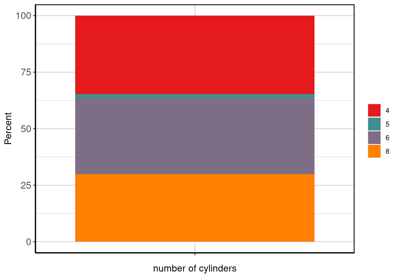
Figure 1: Stacked barplot of number of cylinders.
Categorical By
For a categorical variable with by, we need to specify x, a by variable, and the data.
cylByYearSummaryExample <- data_summary(x = "cyl", by = "year", data = mpg)Show method to output table and plot
show(cylByYearSummaryExample)## number of cylinders 1999 2008 Overall
## 1 4 45 (38.46%) 36 (30.77%) 81 (34.62%)
## 2 5 0 (0%) 4 (3.42%) 4 (1.71%)
## 3 6 45 (38.46%) 34 (29.06%) 79 (33.76%)
## 4 8 27 (23.08%) 43 (36.75%) 70 (29.91%)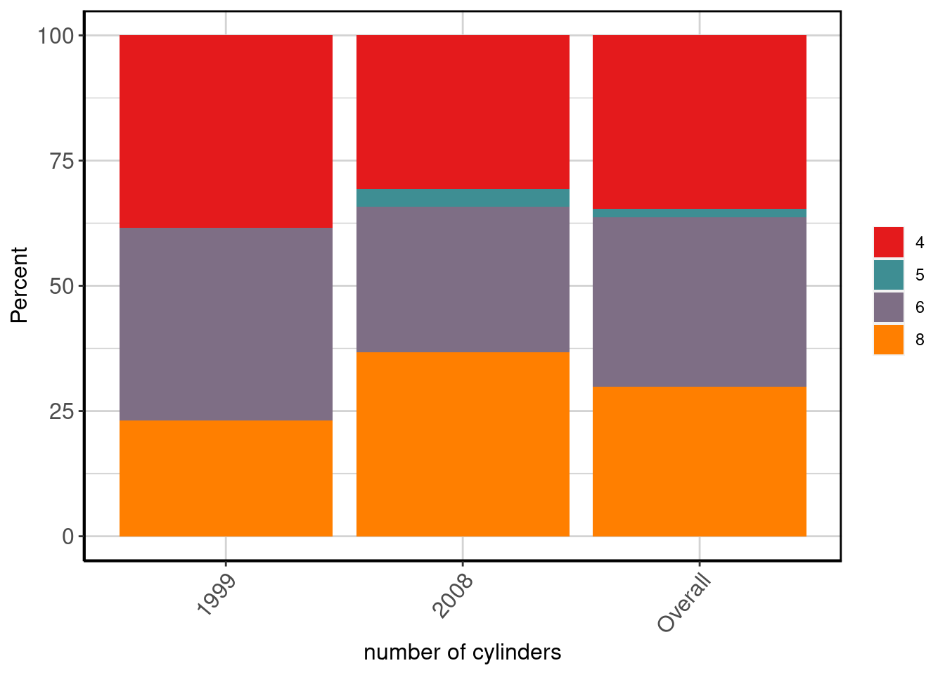
Output the summary table
data_summary_table(cylByYearSummaryExample)## number of cylinders 1999 2008 Overall
## 1 4 45 (38.46%) 36 (30.77%) 81 (34.62%)
## 2 5 0 (0%) 4 (3.42%) 4 (1.71%)
## 3 6 45 (38.46%) 34 (29.06%) 79 (33.76%)
## 4 8 27 (23.08%) 43 (36.75%) 70 (29.91%)Output the plot
data_summary_plot(cylByYearSummaryExample)
Generate a knitr friendly summary table
make_kable_output(cylByYearSummaryExample)| number of cylinders | 1999 | 2008 | Overall |
|---|---|---|---|
| 4 | 45 (38.46%) | 36 (30.77%) | 81 (34.62%) |
| 5 | 0 (0%) | 4 (3.42%) | 4 (1.71%) |
| 6 | 45 (38.46%) | 34 (29.06%) | 79 (33.76%) |
| 8 | 27 (23.08%) | 43 (36.75%) | 70 (29.91%) |
Generate knitr friendly output
make_complete_output(cylByYearSummaryExample)| number of cylinders | 1999 | 2008 | Overall |
|---|---|---|---|
| 4 | 45 (38.46%) | 36 (30.77%) | 81 (34.62%) |
| 5 | 0 (0%) | 4 (3.42%) | 4 (1.71%) |
| 6 | 45 (38.46%) | 34 (29.06%) | 79 (33.76%) |
| 8 | 27 (23.08%) | 43 (36.75%) | 70 (29.91%) |

Figure 2: Stacked barplot of number of cylinders by year of manufacture.
Categorical By By
For a categorical variable with two or more by variables, we need to specify x, the by variables as a character string, and the data.
cylByYearByPartySummaryExample <- data_summary(x = "cyl", by = c("year", "party"), data = mpg)Show method to output table and plot
show(cylByYearByPartySummaryExample)## number of cylinders 1999, republican 2008, republican 1999, democrat
## 1 4 14 (45.16%) 9 (36%) 12 (40%)
## 2 5 0 (0%) 1 (4%) 0 (0%)
## 3 6 12 (38.71%) 5 (20%) 7 (23.33%)
## 4 8 5 (16.13%) 10 (40%) 11 (36.67%)
## 2008, democrat 1999, independent 2008, independent Overall R NA Value
## 1 8 (25.81%) 9 (32.14%) 12 (35.29%) 81 (34.62%) 17 (30.91%)
## 2 2 (6.45%) 0 (0%) 0 (0%) 4 (1.71%) 1 (1.82%)
## 3 6 (19.35%) 13 (46.43%) 12 (35.29%) 79 (33.76%) 24 (43.64%)
## 4 15 (48.39%) 6 (21.43%) 10 (29.41%) 70 (29.91%) 13 (23.64%)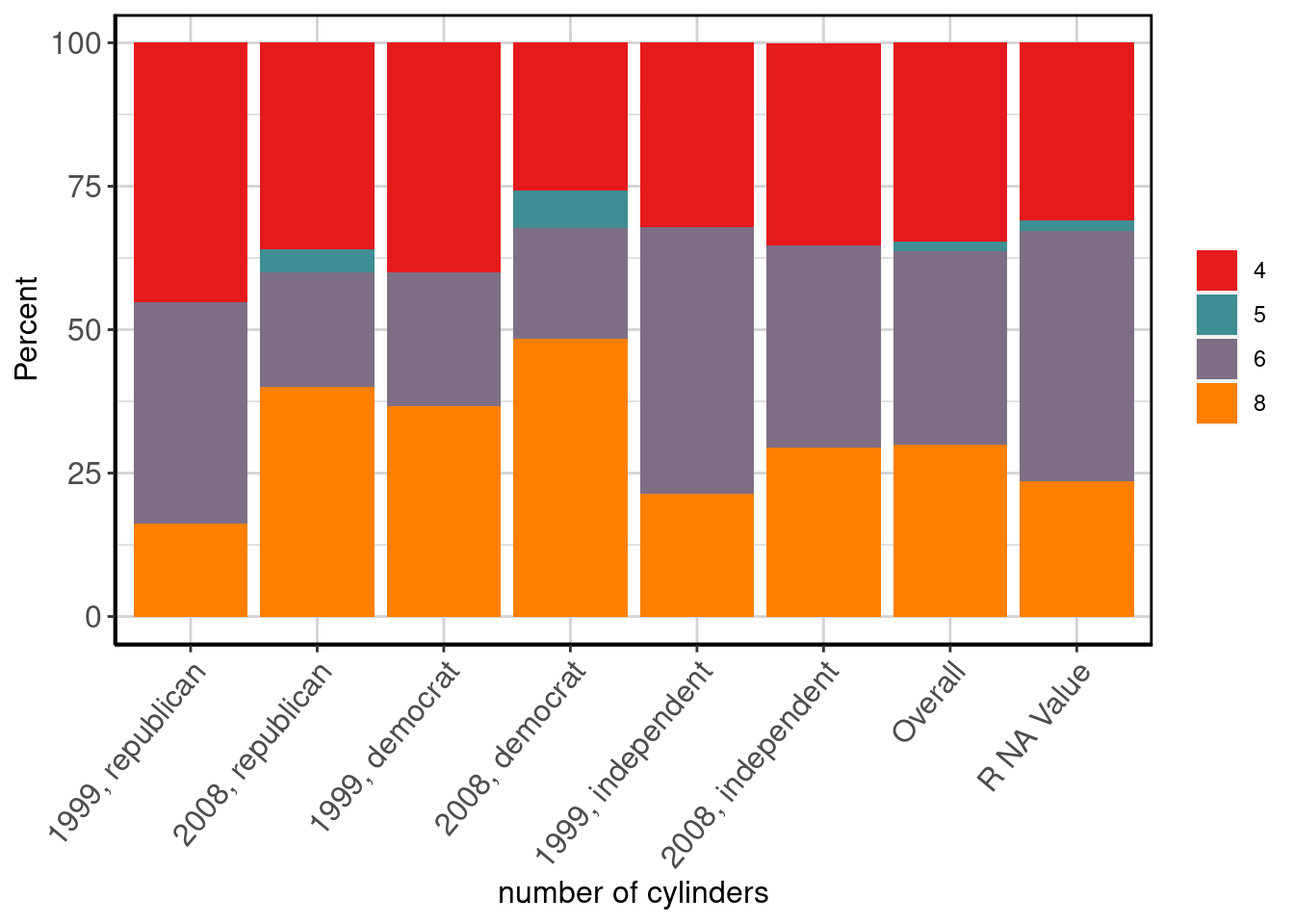
Output the summary table
data_summary_table(cylByYearByPartySummaryExample)## number of cylinders 1999, republican 2008, republican 1999, democrat
## 1 4 14 (45.16%) 9 (36%) 12 (40%)
## 2 5 0 (0%) 1 (4%) 0 (0%)
## 3 6 12 (38.71%) 5 (20%) 7 (23.33%)
## 4 8 5 (16.13%) 10 (40%) 11 (36.67%)
## 2008, democrat 1999, independent 2008, independent Overall R NA Value
## 1 8 (25.81%) 9 (32.14%) 12 (35.29%) 81 (34.62%) 17 (30.91%)
## 2 2 (6.45%) 0 (0%) 0 (0%) 4 (1.71%) 1 (1.82%)
## 3 6 (19.35%) 13 (46.43%) 12 (35.29%) 79 (33.76%) 24 (43.64%)
## 4 15 (48.39%) 6 (21.43%) 10 (29.41%) 70 (29.91%) 13 (23.64%)Output the plot
data_summary_plot(cylByYearByPartySummaryExample)
Generate a knitr friendly summary table
make_kable_output(cylByYearByPartySummaryExample)| number of cylinders | 1999, republican | 2008, republican | 1999, democrat | 2008, democrat | 1999, independent | 2008, independent | Overall | R NA Value |
|---|---|---|---|---|---|---|---|---|
| 4 | 14 (45.16%) | 9 (36%) | 12 (40%) | 8 (25.81%) | 9 (32.14%) | 12 (35.29%) | 81 (34.62%) | 17 (30.91%) |
| 5 | 0 (0%) | 1 (4%) | 0 (0%) | 2 (6.45%) | 0 (0%) | 0 (0%) | 4 (1.71%) | 1 (1.82%) |
| 6 | 12 (38.71%) | 5 (20%) | 7 (23.33%) | 6 (19.35%) | 13 (46.43%) | 12 (35.29%) | 79 (33.76%) | 24 (43.64%) |
| 8 | 5 (16.13%) | 10 (40%) | 11 (36.67%) | 15 (48.39%) | 6 (21.43%) | 10 (29.41%) | 70 (29.91%) | 13 (23.64%) |
Generate knitr friendly output
make_complete_output(cylByYearByPartySummaryExample)| number of cylinders | 1999, republican | 2008, republican | 1999, democrat | 2008, democrat | 1999, independent | 2008, independent | Overall | R NA Value |
|---|---|---|---|---|---|---|---|---|
| 4 | 14 (45.16%) | 9 (36%) | 12 (40%) | 8 (25.81%) | 9 (32.14%) | 12 (35.29%) | 81 (34.62%) | 17 (30.91%) |
| 5 | 0 (0%) | 1 (4%) | 0 (0%) | 2 (6.45%) | 0 (0%) | 0 (0%) | 4 (1.71%) | 1 (1.82%) |
| 6 | 12 (38.71%) | 5 (20%) | 7 (23.33%) | 6 (19.35%) | 13 (46.43%) | 12 (35.29%) | 79 (33.76%) | 24 (43.64%) |
| 8 | 5 (16.13%) | 10 (40%) | 11 (36.67%) | 15 (48.39%) | 6 (21.43%) | 10 (29.41%) | 70 (29.91%) | 13 (23.64%) |

Figure 3: Stacked barplot of number of cylinders by year of manufacture by some random political parties.
Continuous
For a continuous variable x, we only need to specify x and the data.
ctySummaryExample <- data_summary(x = "cty", data = mpg)Show method to output table and plot
show(ctySummaryExample)## Label N P NA Mean S Dev Med MAD 25th P 75th P IQR Min
## 1 city miles per gallon 234 0 16.86 4.26 17 4.45 14 19 5 9
## Max
## 1 35
Output the summary table
data_summary_table(ctySummaryExample)## Label N P NA Mean S Dev Med MAD 25th P 75th P IQR Min
## 1 city miles per gallon 234 0 16.86 4.26 17 4.45 14 19 5 9
## Max
## 1 35Output the plot
data_summary_plot(ctySummaryExample)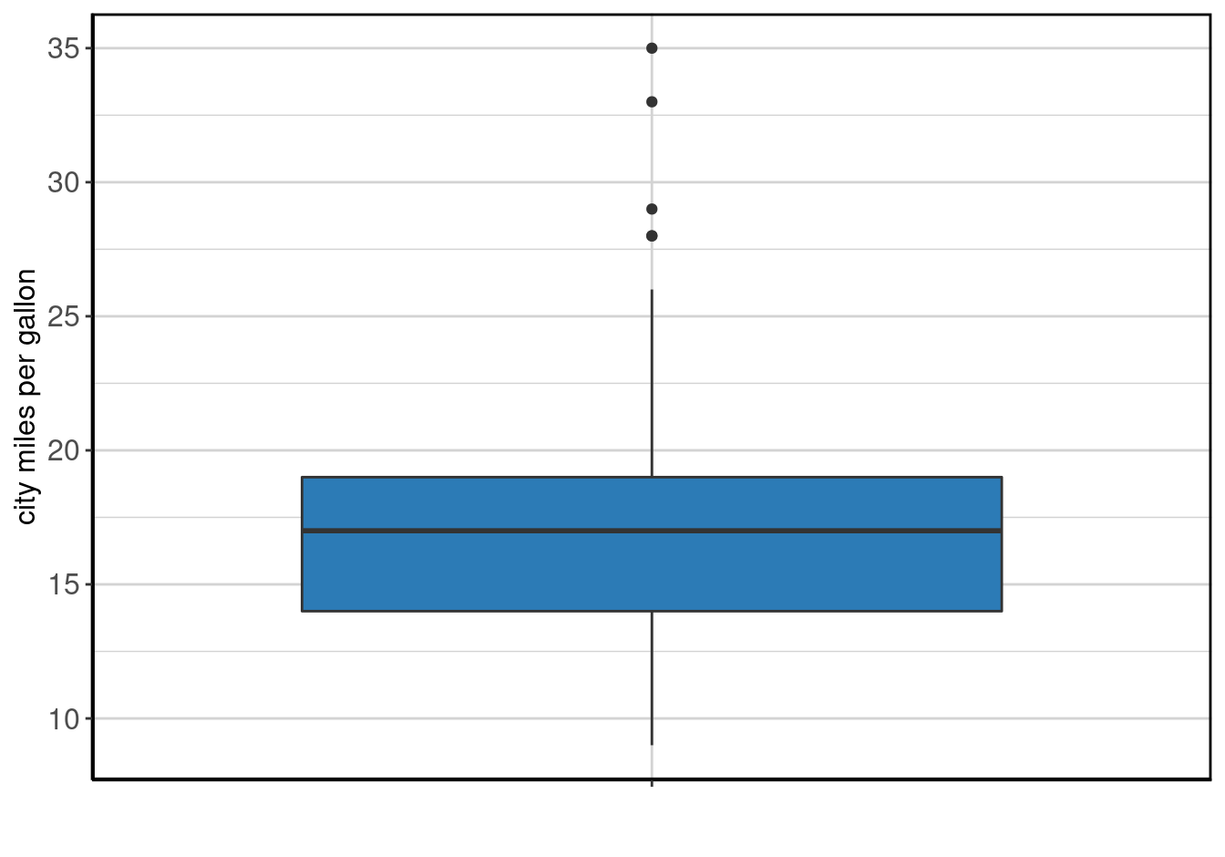
Generate knitr friendly summary table
make_kable_output(ctySummaryExample)| Label | N | P NA | Mean | S Dev | Med | MAD | 25th P | 75th P | IQR | Min | Max | |
|---|---|---|---|---|---|---|---|---|---|---|---|---|
| city miles per gallon | 234 | 0 | 16.86 | 4.26 | 17 | 4.45 | 14 | 19 | 5 | 9 | 35 |
Generate knitr friendly output
make_complete_output(ctySummaryExample)| Label | N | P NA | Mean | S Dev | Med | MAD | 25th P | 75th P | IQR | Min | Max | |
|---|---|---|---|---|---|---|---|---|---|---|---|---|
| city miles per gallon | 234 | 0 | 16.86 | 4.26 | 17 | 4.45 | 14 | 19 | 5 | 9 | 35 |

Figure 4: Stacked barplot of city miles per gallon.
Continuous By
For a continuous variable with by, we need to specify x, a by variable, and the data.
ctyByCylSummaryExample <- data_summary(x = "cty", by = "cyl", data = mpg)Show method to output table and plot
show(ctyByCylSummaryExample)## number of cylinders Label N P NA Mean S Dev Med MAD
## 1 4 city miles per gallon 81 0 21.01 3.50 21.0 2.97
## 2 5 city miles per gallon 4 0 20.50 0.58 20.5 0.74
## 3 6 city miles per gallon 79 0 16.22 1.77 16.0 1.48
## 4 8 city miles per gallon 70 0 12.57 1.81 13.0 2.22
## 5 Overall city miles per gallon 234 0 16.86 4.26 17.0 4.45
## 25th P 75th P IQR Min Max
## 1 19 22 3 15 35
## 2 20 21 1 20 21
## 3 15 18 3 11 19
## 4 11 14 3 9 16
## 5 14 19 5 9 35
Output the summary table
data_summary_table(ctyByCylSummaryExample)## number of cylinders Label N P NA Mean S Dev Med MAD
## 1 4 city miles per gallon 81 0 21.01 3.50 21.0 2.97
## 2 5 city miles per gallon 4 0 20.50 0.58 20.5 0.74
## 3 6 city miles per gallon 79 0 16.22 1.77 16.0 1.48
## 4 8 city miles per gallon 70 0 12.57 1.81 13.0 2.22
## 5 Overall city miles per gallon 234 0 16.86 4.26 17.0 4.45
## 25th P 75th P IQR Min Max
## 1 19 22 3 15 35
## 2 20 21 1 20 21
## 3 15 18 3 11 19
## 4 11 14 3 9 16
## 5 14 19 5 9 35Output the plot
data_summary_plot(ctyByCylSummaryExample)
Generate a knitr friendly summary table
make_kable_output(ctyByCylSummaryExample)| number of cylinders | Label | N | P NA | Mean | S Dev | Med | MAD | 25th P | 75th P | IQR | Min | Max |
|---|---|---|---|---|---|---|---|---|---|---|---|---|
| 4 | city miles per gallon | 81 | 0 | 21.01 | 3.50 | 21.0 | 2.97 | 19 | 22 | 3 | 15 | 35 |
| 5 | city miles per gallon | 4 | 0 | 20.50 | 0.58 | 20.5 | 0.74 | 20 | 21 | 1 | 20 | 21 |
| 6 | city miles per gallon | 79 | 0 | 16.22 | 1.77 | 16.0 | 1.48 | 15 | 18 | 3 | 11 | 19 |
| 8 | city miles per gallon | 70 | 0 | 12.57 | 1.81 | 13.0 | 2.22 | 11 | 14 | 3 | 9 | 16 |
| Overall | city miles per gallon | 234 | 0 | 16.86 | 4.26 | 17.0 | 4.45 | 14 | 19 | 5 | 9 | 35 |
Generate knitr friendly output
make_complete_output(ctyByCylSummaryExample)| number of cylinders | Label | N | P NA | Mean | S Dev | Med | MAD | 25th P | 75th P | IQR | Min | Max |
|---|---|---|---|---|---|---|---|---|---|---|---|---|
| 4 | city miles per gallon | 81 | 0 | 21.01 | 3.50 | 21.0 | 2.97 | 19 | 22 | 3 | 15 | 35 |
| 5 | city miles per gallon | 4 | 0 | 20.50 | 0.58 | 20.5 | 0.74 | 20 | 21 | 1 | 20 | 21 |
| 6 | city miles per gallon | 79 | 0 | 16.22 | 1.77 | 16.0 | 1.48 | 15 | 18 | 3 | 11 | 19 |
| 8 | city miles per gallon | 70 | 0 | 12.57 | 1.81 | 13.0 | 2.22 | 11 | 14 | 3 | 9 | 16 |
| Overall | city miles per gallon | 234 | 0 | 16.86 | 4.26 | 17.0 | 4.45 | 14 | 19 | 5 | 9 | 35 |
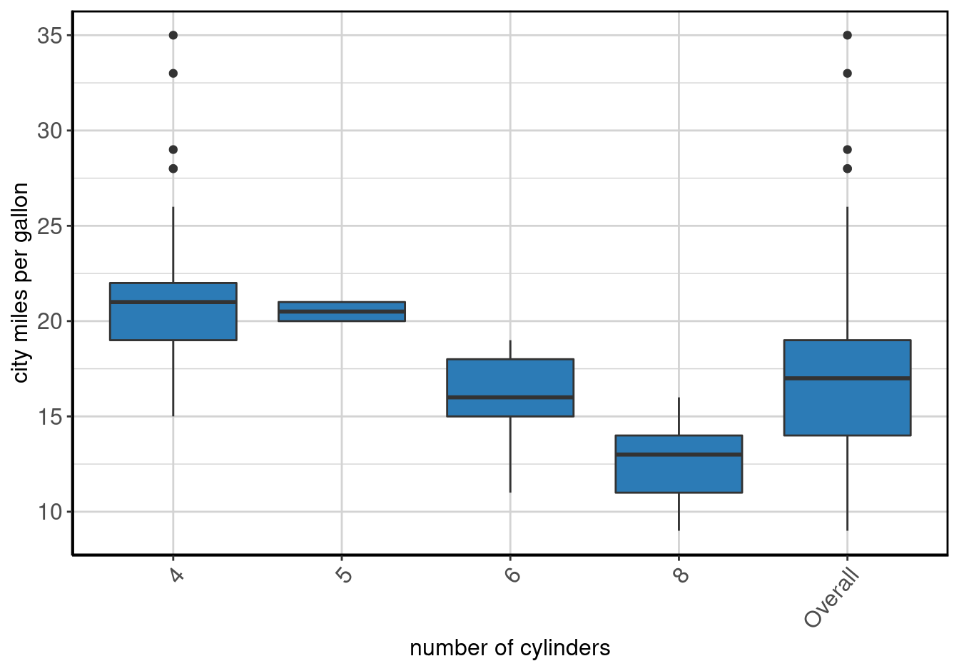
Figure 5: Stacked barplot of city miles per gallon by number of cylinders.
Continuous By By
For a continuous variable with two or more by variables, we need to specify x, the by variables as a character string, and the data.
ctyByCylByYearSummaryExample <- data_summary(x = "cty", by = c("cyl", "year"), data = mpg)Show method to output table and plot
show(ctyByCylByYearSummaryExample)## number of cylinders by year of manufacture Label N P NA
## 1 4, 1999 city miles per gallon 45 0
## 2 6, 1999 city miles per gallon 45 0
## 3 8, 1999 city miles per gallon 27 0
## 4 4, 2008 city miles per gallon 36 0
## 5 5, 2008 city miles per gallon 4 0
## 6 6, 2008 city miles per gallon 34 0
## 7 8, 2008 city miles per gallon 43 0
## 8 Overall city miles per gallon 234 0
## Mean S Dev Med MAD 25th P 75th P IQR Min Max
## 1 20.84 4.24 19.0 2.97 18 21 3.0 15 35
## 2 16.07 1.67 16.0 2.97 15 18 3.0 13 19
## 3 12.22 1.65 11.0 0.00 11 13 2.0 11 16
## 4 21.22 2.29 21.0 1.48 20 22 2.0 17 28
## 5 20.50 0.58 20.5 0.74 20 21 1.0 20 21
## 6 16.41 1.91 17.0 1.48 15 18 2.5 11 19
## 7 12.79 1.88 13.0 1.48 12 14 2.0 9 16
## 8 16.86 4.26 17.0 4.45 14 19 5.0 9 35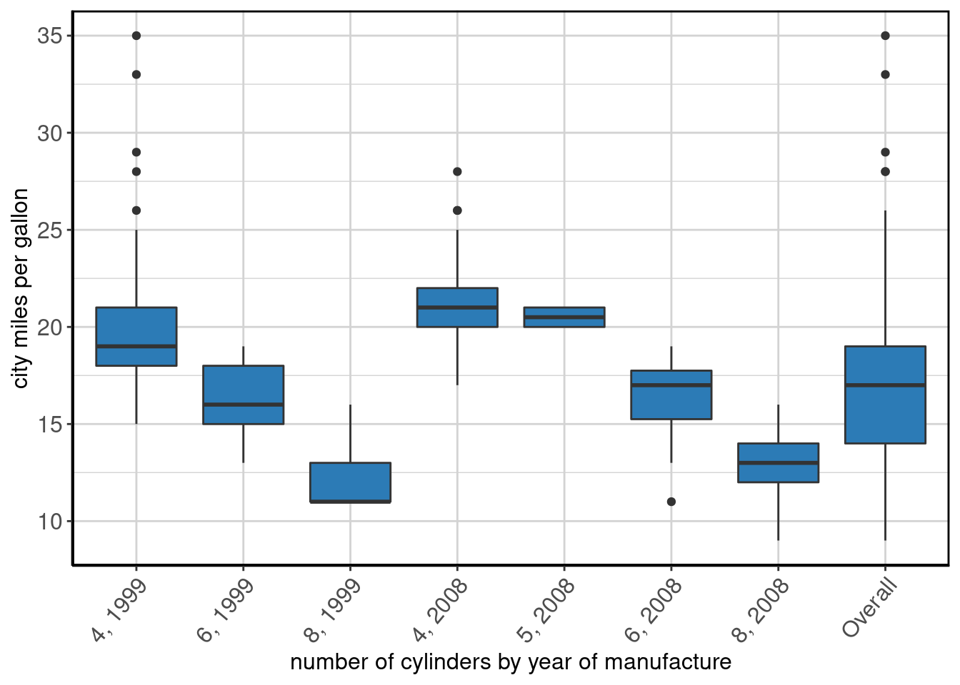
Output the summary table
data_summary_table(ctyByCylByYearSummaryExample)## number of cylinders by year of manufacture Label N P NA
## 1 4, 1999 city miles per gallon 45 0
## 2 6, 1999 city miles per gallon 45 0
## 3 8, 1999 city miles per gallon 27 0
## 4 4, 2008 city miles per gallon 36 0
## 5 5, 2008 city miles per gallon 4 0
## 6 6, 2008 city miles per gallon 34 0
## 7 8, 2008 city miles per gallon 43 0
## 8 Overall city miles per gallon 234 0
## Mean S Dev Med MAD 25th P 75th P IQR Min Max
## 1 20.84 4.24 19.0 2.97 18 21 3.0 15 35
## 2 16.07 1.67 16.0 2.97 15 18 3.0 13 19
## 3 12.22 1.65 11.0 0.00 11 13 2.0 11 16
## 4 21.22 2.29 21.0 1.48 20 22 2.0 17 28
## 5 20.50 0.58 20.5 0.74 20 21 1.0 20 21
## 6 16.41 1.91 17.0 1.48 15 18 2.5 11 19
## 7 12.79 1.88 13.0 1.48 12 14 2.0 9 16
## 8 16.86 4.26 17.0 4.45 14 19 5.0 9 35Output the plot
data_summary_plot(ctyByCylByYearSummaryExample)
Generate a knitr friendly summary table
make_kable_output(ctyByCylByYearSummaryExample)| number of cylinders by year of manufacture | Label | N | P NA | Mean | S Dev | Med | MAD | 25th P | 75th P | IQR | Min | Max |
|---|---|---|---|---|---|---|---|---|---|---|---|---|
| 4, 1999 | city miles per gallon | 45 | 0 | 20.84 | 4.24 | 19.0 | 2.97 | 18 | 21 | 3.0 | 15 | 35 |
| 6, 1999 | city miles per gallon | 45 | 0 | 16.07 | 1.67 | 16.0 | 2.97 | 15 | 18 | 3.0 | 13 | 19 |
| 8, 1999 | city miles per gallon | 27 | 0 | 12.22 | 1.65 | 11.0 | 0.00 | 11 | 13 | 2.0 | 11 | 16 |
| 4, 2008 | city miles per gallon | 36 | 0 | 21.22 | 2.29 | 21.0 | 1.48 | 20 | 22 | 2.0 | 17 | 28 |
| 5, 2008 | city miles per gallon | 4 | 0 | 20.50 | 0.58 | 20.5 | 0.74 | 20 | 21 | 1.0 | 20 | 21 |
| 6, 2008 | city miles per gallon | 34 | 0 | 16.41 | 1.91 | 17.0 | 1.48 | 15 | 18 | 2.5 | 11 | 19 |
| 8, 2008 | city miles per gallon | 43 | 0 | 12.79 | 1.88 | 13.0 | 1.48 | 12 | 14 | 2.0 | 9 | 16 |
| Overall | city miles per gallon | 234 | 0 | 16.86 | 4.26 | 17.0 | 4.45 | 14 | 19 | 5.0 | 9 | 35 |
Generate knitr friendly output
make_complete_output(ctyByCylByYearSummaryExample)| number of cylinders by year of manufacture | Label | N | P NA | Mean | S Dev | Med | MAD | 25th P | 75th P | IQR | Min | Max |
|---|---|---|---|---|---|---|---|---|---|---|---|---|
| 4, 1999 | city miles per gallon | 45 | 0 | 20.84 | 4.24 | 19.0 | 2.97 | 18 | 21 | 3.0 | 15 | 35 |
| 6, 1999 | city miles per gallon | 45 | 0 | 16.07 | 1.67 | 16.0 | 2.97 | 15 | 18 | 3.0 | 13 | 19 |
| 8, 1999 | city miles per gallon | 27 | 0 | 12.22 | 1.65 | 11.0 | 0.00 | 11 | 13 | 2.0 | 11 | 16 |
| 4, 2008 | city miles per gallon | 36 | 0 | 21.22 | 2.29 | 21.0 | 1.48 | 20 | 22 | 2.0 | 17 | 28 |
| 5, 2008 | city miles per gallon | 4 | 0 | 20.50 | 0.58 | 20.5 | 0.74 | 20 | 21 | 1.0 | 20 | 21 |
| 6, 2008 | city miles per gallon | 34 | 0 | 16.41 | 1.91 | 17.0 | 1.48 | 15 | 18 | 2.5 | 11 | 19 |
| 8, 2008 | city miles per gallon | 43 | 0 | 12.79 | 1.88 | 13.0 | 1.48 | 12 | 14 | 2.0 | 9 | 16 |
| Overall | city miles per gallon | 234 | 0 | 16.86 | 4.26 | 17.0 | 4.45 | 14 | 19 | 5.0 | 9 | 35 |

Figure 6: Stacked barplot of city miles per gallon by number of cylinders by year of manufacture.
Date
For a date variable x, we need to specify x, the data, and difftime_units.
dpSummaryExample <- data_summary(x = "dp", data = mpg[which(mpg$dp != "1000-05-02" | is.na(mpg$dp)), ], difftime_units = "weeks")Show method to output table and plot
show(dpSummaryExample)## Label N P NA Mean S Dev Med
## 1 date of purchase (Date class) 213 8.58 2003-12-21 236.59 weeks 1999-12-24
## MAD 25th P 75th P IQR Min Max
## 1 74.98 weeks 1999-07-14 2008-09-01 476.7143 weeks 1999-01-04 2008-12-23
Output the summary table
data_summary_table(dpSummaryExample)## Label N P NA Mean S Dev Med
## 1 date of purchase (Date class) 213 8.58 2003-12-21 236.59 weeks 1999-12-24
## MAD 25th P 75th P IQR Min Max
## 1 74.98 weeks 1999-07-14 2008-09-01 476.7143 weeks 1999-01-04 2008-12-23Output the plot
data_summary_plot(dpSummaryExample)
Generate knitr friendly summary table
make_kable_output(dpSummaryExample)| Label | N | P NA | Mean | S Dev | Med | MAD | 25th P | 75th P | IQR | Min | Max | |
|---|---|---|---|---|---|---|---|---|---|---|---|---|
| date of purchase (Date class) | 213 | 8.58 | 2003-12-21 | 236.59 weeks | 1999-12-24 | 74.98 weeks | 1999-07-14 | 2008-09-01 | 476.7143 weeks | 1999-01-04 | 2008-12-23 |
Generate knitr friendly output
make_complete_output(dpSummaryExample)| Label | N | P NA | Mean | S Dev | Med | MAD | 25th P | 75th P | IQR | Min | Max | |
|---|---|---|---|---|---|---|---|---|---|---|---|---|
| date of purchase (Date class) | 213 | 8.58 | 2003-12-21 | 236.59 weeks | 1999-12-24 | 74.98 weeks | 1999-07-14 | 2008-09-01 | 476.7143 weeks | 1999-01-04 | 2008-12-23 |

Figure 7: Stacked barplot of date of purchase (Date class).
Date By
For a date variable with by, we need to specify x, a by variable, the data, and difftime_units.
dpByCylSummaryExample <- data_summary(x = "dp", by = "cyl", data = mpg[which(mpg$dp != "1000-05-02" | is.na(mpg$dp)), ], difftime_units = "weeks")Show method to output table and plot
show(dpByCylSummaryExample)## number of cylinders Label N P NA Mean
## 1 4 date of purchase (Date class) 73 8.75 2003-03-03
## 2 5 date of purchase (Date class) 3 25.00 2008-09-25
## 3 6 date of purchase (Date class) 71 10.13 2003-06-14
## 4 8 date of purchase (Date class) 66 5.71 2005-03-13
## 5 Overall date of purchase (Date class) 213 8.58 2003-12-21
## S Dev Med MAD 25th P 75th P IQR
## 1 234.04 weeks 1999-10-11 49.35 weeks 1999-06-03 2008-07-28 477.57143 weeks
## 2 16.08 weeks 2008-11-13 6.78 weeks 2008-05-20 2008-12-15 29.85714 weeks
## 3 235.29 weeks 1999-11-02 50.20 weeks 1999-07-14 2008-08-02 472.42857 weeks
## 4 229.06 weeks 2008-02-10 52.42 weeks 1999-10-04 2008-09-08 466.00000 weeks
## 5 236.59 weeks 1999-12-24 74.98 weeks 1999-07-14 2008-09-01 476.71429 weeks
## Min Max
## 1 1999-01-14 2008-12-23
## 2 2008-05-20 2008-12-15
## 3 1999-01-05 2008-12-09
## 4 1999-01-04 2008-12-14
## 5 1999-01-04 2008-12-23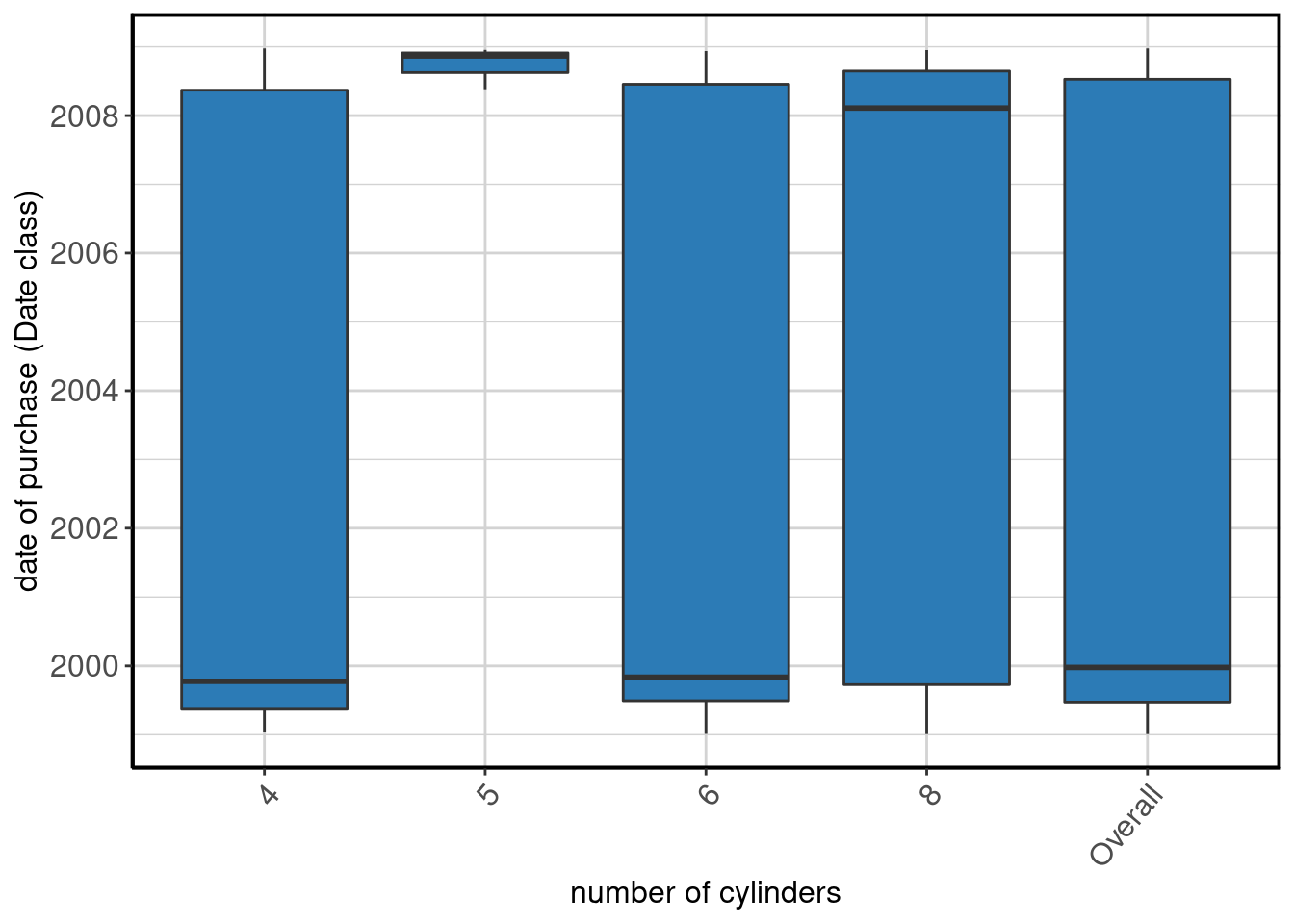
Output the summary table
data_summary_table(dpByCylSummaryExample)## number of cylinders Label N P NA Mean
## 1 4 date of purchase (Date class) 73 8.75 2003-03-03
## 2 5 date of purchase (Date class) 3 25.00 2008-09-25
## 3 6 date of purchase (Date class) 71 10.13 2003-06-14
## 4 8 date of purchase (Date class) 66 5.71 2005-03-13
## 5 Overall date of purchase (Date class) 213 8.58 2003-12-21
## S Dev Med MAD 25th P 75th P IQR
## 1 234.04 weeks 1999-10-11 49.35 weeks 1999-06-03 2008-07-28 477.57143 weeks
## 2 16.08 weeks 2008-11-13 6.78 weeks 2008-05-20 2008-12-15 29.85714 weeks
## 3 235.29 weeks 1999-11-02 50.20 weeks 1999-07-14 2008-08-02 472.42857 weeks
## 4 229.06 weeks 2008-02-10 52.42 weeks 1999-10-04 2008-09-08 466.00000 weeks
## 5 236.59 weeks 1999-12-24 74.98 weeks 1999-07-14 2008-09-01 476.71429 weeks
## Min Max
## 1 1999-01-14 2008-12-23
## 2 2008-05-20 2008-12-15
## 3 1999-01-05 2008-12-09
## 4 1999-01-04 2008-12-14
## 5 1999-01-04 2008-12-23Output the plot
data_summary_plot(dpByCylSummaryExample)
Generate a knitr friendly summary table
make_kable_output(dpByCylSummaryExample)| number of cylinders | Label | N | P NA | Mean | S Dev | Med | MAD | 25th P | 75th P | IQR | Min | Max |
|---|---|---|---|---|---|---|---|---|---|---|---|---|
| 4 | date of purchase (Date class) | 73 | 8.75 | 2003-03-03 | 234.04 weeks | 1999-10-11 | 49.35 weeks | 1999-06-03 | 2008-07-28 | 477.57143 weeks | 1999-01-14 | 2008-12-23 |
| 5 | date of purchase (Date class) | 3 | 25.00 | 2008-09-25 | 16.08 weeks | 2008-11-13 | 6.78 weeks | 2008-05-20 | 2008-12-15 | 29.85714 weeks | 2008-05-20 | 2008-12-15 |
| 6 | date of purchase (Date class) | 71 | 10.13 | 2003-06-14 | 235.29 weeks | 1999-11-02 | 50.20 weeks | 1999-07-14 | 2008-08-02 | 472.42857 weeks | 1999-01-05 | 2008-12-09 |
| 8 | date of purchase (Date class) | 66 | 5.71 | 2005-03-13 | 229.06 weeks | 2008-02-10 | 52.42 weeks | 1999-10-04 | 2008-09-08 | 466.00000 weeks | 1999-01-04 | 2008-12-14 |
| Overall | date of purchase (Date class) | 213 | 8.58 | 2003-12-21 | 236.59 weeks | 1999-12-24 | 74.98 weeks | 1999-07-14 | 2008-09-01 | 476.71429 weeks | 1999-01-04 | 2008-12-23 |
Generate knitr friendly output
make_complete_output(dpByCylSummaryExample)| number of cylinders | Label | N | P NA | Mean | S Dev | Med | MAD | 25th P | 75th P | IQR | Min | Max |
|---|---|---|---|---|---|---|---|---|---|---|---|---|
| 4 | date of purchase (Date class) | 73 | 8.75 | 2003-03-03 | 234.04 weeks | 1999-10-11 | 49.35 weeks | 1999-06-03 | 2008-07-28 | 477.57143 weeks | 1999-01-14 | 2008-12-23 |
| 5 | date of purchase (Date class) | 3 | 25.00 | 2008-09-25 | 16.08 weeks | 2008-11-13 | 6.78 weeks | 2008-05-20 | 2008-12-15 | 29.85714 weeks | 2008-05-20 | 2008-12-15 |
| 6 | date of purchase (Date class) | 71 | 10.13 | 2003-06-14 | 235.29 weeks | 1999-11-02 | 50.20 weeks | 1999-07-14 | 2008-08-02 | 472.42857 weeks | 1999-01-05 | 2008-12-09 |
| 8 | date of purchase (Date class) | 66 | 5.71 | 2005-03-13 | 229.06 weeks | 2008-02-10 | 52.42 weeks | 1999-10-04 | 2008-09-08 | 466.00000 weeks | 1999-01-04 | 2008-12-14 |
| Overall | date of purchase (Date class) | 213 | 8.58 | 2003-12-21 | 236.59 weeks | 1999-12-24 | 74.98 weeks | 1999-07-14 | 2008-09-01 | 476.71429 weeks | 1999-01-04 | 2008-12-23 |
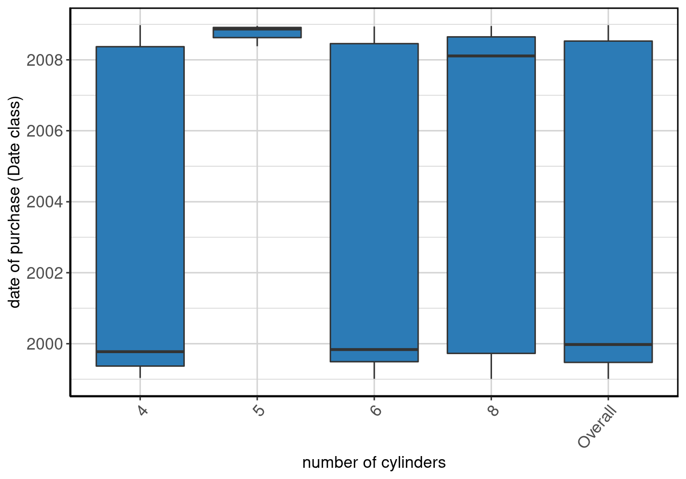
Figure 8: Stacked barplot of date of purchase (Date class) by number of cylinders.
Date By By
For a date variable with two or more by variables, we need to specify x, the by variables as a character string, the data, and difftime_units.
dpByCylByCommentsSummaryExample <- data_summary(x = "dp", by = c("cyl", "comments"), data = mpg[which(mpg$dp != "1000-05-02" | is.na(mpg$dp)), ], difftime_units = "weeks")Show method to output table and plot
show(dpByCylByCommentsSummaryExample)## number of cylinders by some random comments
## 1 4, .
## 2 6, .
## 3 8, .
## 4 4, Blah, Blah, Blah, Blah, Blah, Blah, Blah, Blah
## 5 6, Blah, Blah, Blah, Blah, Blah, Blah, Blah, Blah
## 6 8, Blah, Blah, Blah, Blah, Blah, Blah, Blah, Blah
## 7 4, Does it also fly?
## 8 6, Does it also fly?
## 9 8, Does it also fly?
## 10 4, Does it come in green?
## 11 6, Does it come in green?
## 12 8, Does it come in green?
## 13 4, I like this car!
## 14 6, I like this car!
## 15 8, I like this car!
## 16 4, Meh.
## 17 6, Meh.
## 18 8, Meh.
## 19 4, Missing
## 20 6, Missing
## 21 8, Missing
## 22 4, This is the worst car ever!
## 23 6, This is the worst car ever!
## 24 8, This is the worst car ever!
## 25 4, want cheese flavoured cars.
## 26 6, want cheese flavoured cars.
## 27 8, want cheese flavoured cars.
## 28 Overall
## 29 R NA Value
## Label N P NA Mean S Dev Med
## 1 date of purchase (Date class) 5 0.00 2003-01-27 252.39 weeks 1999-10-26
## 2 date of purchase (Date class) 9 0.00 2004-08-21 241.15 weeks 2008-04-02
## 3 date of purchase (Date class) 10 9.09 2004-11-28 246.03 weeks 2008-02-07
## 4 date of purchase (Date class) 9 0.00 2002-08-10 241.71 weeks 1999-09-12
## 5 date of purchase (Date class) 7 12.50 2004-08-16 254.96 weeks 2008-05-13
## 6 date of purchase (Date class) 4 0.00 2004-01-07 274.68 weeks 2004-02-23
## 7 date of purchase (Date class) 5 0.00 2002-12-14 265.47 weeks 1999-08-06
## 8 date of purchase (Date class) 4 42.86 2001-09-28 225.84 weeks 1999-08-23
## 9 date of purchase (Date class) 4 0.00 2004-03-25 272.68 weeks 2004-04-06
## 10 date of purchase (Date class) 15 0.00 2003-07-23 243.88 weeks 1999-08-26
## 11 date of purchase (Date class) 3 0.00 2002-06-23 268.42 weeks 1999-09-09
## 12 date of purchase (Date class) 5 0.00 2006-07-09 217.62 weeks 2008-02-09
## 13 date of purchase (Date class) 8 11.11 2005-04-06 247.72 weeks 2008-07-29
## 14 date of purchase (Date class) 7 22.22 2002-01-30 232.78 weeks 1999-08-23
## 15 date of purchase (Date class) 4 0.00 2001-11-20 246.39 weeks 1999-09-27
## 16 date of purchase (Date class) 6 0.00 1999-05-01 9.86 weeks 1999-04-25
## 17 date of purchase (Date class) 6 0.00 2005-06-05 248.14 weeks 2008-04-27
## 18 date of purchase (Date class) 5 16.67 2008-04-14 9.80 weeks 2008-04-15
## 19 date of purchase (Date class) 3 50.00 2002-08-26 280.92 weeks 1999-10-09
## 20 date of purchase (Date class) 5 0.00 2004-12-23 255.73 weeks 2008-05-24
## 21 date of purchase (Date class) 14 0.00 2005-11-13 226.66 weeks 2008-04-02
## 22 date of purchase (Date class) 7 0.00 2003-05-28 247.48 weeks 1999-11-24
## 23 date of purchase (Date class) 9 10.00 2002-08-03 237.70 weeks 1999-10-18
## 24 date of purchase (Date class) 5 0.00 2006-09-25 213.60 weeks 2008-07-04
## 25 date of purchase (Date class) 10 9.09 2003-02-13 238.91 weeks 1999-12-10
## 26 date of purchase (Date class) 13 0.00 2002-04-09 231.98 weeks 1999-08-31
## 27 date of purchase (Date class) 8 11.11 2005-01-02 240.53 weeks 2008-02-06
## 28 date of purchase (Date class) 213 8.58 2003-12-21 236.59 weeks 1999-12-24
## 29 date of purchase (Date class) 20 16.67 2003-12-06 236.95 weeks 2003-12-24
## MAD 25th P 75th P IQR Min Max
## 1 54.64 weeks 1999-02-10 2008-02-08 469.285714 weeks 1999-02-10 2008-08-12
## 2 44.27 weeks 1999-08-28 2008-06-18 459.571429 weeks 1999-07-14 2008-10-28
## 3 61.53 weeks 1999-10-05 2008-09-06 465.571429 weeks 1999-01-13 2008-11-27
## 4 38.34 weeks 1999-03-15 2008-05-25 479.857143 weeks 1999-03-08 2008-12-23
## 5 31.13 weeks 1999-06-07 2008-08-02 477.714286 weeks 1999-03-19 2008-10-07
## 6 342.16 weeks 1999-02-03 2008-06-12 488.142857 weeks 1999-02-03 2008-09-09
## 7 43.21 weeks 1999-01-14 2008-02-14 474.000000 weeks 1999-01-14 2008-11-26
## 8 12.71 weeks 1999-07-03 <NA> NA weeks 1999-06-15 2008-03-25
## 9 347.46 weeks 1999-07-16 2008-08-25 475.428571 weeks 1999-07-16 2008-11-10
## 10 47.02 weeks 1999-03-24 2008-02-26 465.857143 weeks 1999-01-16 2008-10-13
## 11 27.75 weeks 1999-05-01 1999-09-09 18.714286 weeks 1999-05-01 2008-05-31
## 12 24.15 weeks 1999-02-01 2008-06-02 487.000000 weeks 1999-02-01 2008-12-08
## 13 20.33 weeks 1999-06-23 2008-09-23 482.857143 weeks 1999-06-08 2008-12-12
## 14 25.84 weeks 1999-04-23 2008-09-05 489.000000 weeks 1999-03-13 2008-09-05
## 15 30.61 weeks 1999-02-12 1999-11-28 41.285714 weeks 1999-02-12 2008-12-14
## 16 8.47 weeks 1999-03-26 1999-05-16 7.285714 weeks 1999-01-25 1999-08-11
## 17 26.58 weeks 1999-07-31 2008-05-08 457.714286 weeks 1999-01-05 2008-09-26
## 18 11.44 weeks 2008-02-21 2008-05-27 13.714286 weeks 2008-01-27 2008-07-13
## 19 34.74 weeks 1999-10-09 <NA> NA weeks 1999-04-28 2008-11-11
## 20 21.18 weeks 1999-07-30 2008-08-09 471.142857 weeks 1999-07-30 2008-09-01
## 21 38.55 weeks 1999-10-04 2008-09-08 466.000000 weeks 1999-01-04 2008-11-15
## 22 50.62 weeks 1999-06-03 2008-02-10 453.428571 weeks 1999-03-30 2008-09-29
## 23 38.34 weeks 1999-04-20 2008-09-13 490.571429 weeks 1999-03-22 2008-10-26
## 24 16.10 weeks 1999-06-02 2008-09-18 485.142857 weeks 1999-06-02 2008-09-19
## 25 57.50 weeks 1999-06-09 2008-05-15 466.142857 weeks 1999-02-17 2008-10-31
## 26 36.85 weeks 1999-03-10 2008-06-24 484.857143 weeks 1999-01-26 2008-12-09
## 27 44.16 weeks 1999-05-21 2008-07-18 478.000000 weeks 1999-04-01 2008-10-18
## 28 74.98 weeks 1999-07-14 2008-09-01 476.714286 weeks 1999-01-04 2008-12-23
## 29 337.72 weeks 1999-08-14 2008-06-25 462.571429 weeks 1999-01-07 2008-12-03
Output the summary table
data_summary_table(dpByCylByCommentsSummaryExample)## number of cylinders by some random comments
## 1 4, .
## 2 6, .
## 3 8, .
## 4 4, Blah, Blah, Blah, Blah, Blah, Blah, Blah, Blah
## 5 6, Blah, Blah, Blah, Blah, Blah, Blah, Blah, Blah
## 6 8, Blah, Blah, Blah, Blah, Blah, Blah, Blah, Blah
## 7 4, Does it also fly?
## 8 6, Does it also fly?
## 9 8, Does it also fly?
## 10 4, Does it come in green?
## 11 6, Does it come in green?
## 12 8, Does it come in green?
## 13 4, I like this car!
## 14 6, I like this car!
## 15 8, I like this car!
## 16 4, Meh.
## 17 6, Meh.
## 18 8, Meh.
## 19 4, Missing
## 20 6, Missing
## 21 8, Missing
## 22 4, This is the worst car ever!
## 23 6, This is the worst car ever!
## 24 8, This is the worst car ever!
## 25 4, want cheese flavoured cars.
## 26 6, want cheese flavoured cars.
## 27 8, want cheese flavoured cars.
## 28 Overall
## 29 R NA Value
## Label N P NA Mean S Dev Med
## 1 date of purchase (Date class) 5 0.00 2003-01-27 252.39 weeks 1999-10-26
## 2 date of purchase (Date class) 9 0.00 2004-08-21 241.15 weeks 2008-04-02
## 3 date of purchase (Date class) 10 9.09 2004-11-28 246.03 weeks 2008-02-07
## 4 date of purchase (Date class) 9 0.00 2002-08-10 241.71 weeks 1999-09-12
## 5 date of purchase (Date class) 7 12.50 2004-08-16 254.96 weeks 2008-05-13
## 6 date of purchase (Date class) 4 0.00 2004-01-07 274.68 weeks 2004-02-23
## 7 date of purchase (Date class) 5 0.00 2002-12-14 265.47 weeks 1999-08-06
## 8 date of purchase (Date class) 4 42.86 2001-09-28 225.84 weeks 1999-08-23
## 9 date of purchase (Date class) 4 0.00 2004-03-25 272.68 weeks 2004-04-06
## 10 date of purchase (Date class) 15 0.00 2003-07-23 243.88 weeks 1999-08-26
## 11 date of purchase (Date class) 3 0.00 2002-06-23 268.42 weeks 1999-09-09
## 12 date of purchase (Date class) 5 0.00 2006-07-09 217.62 weeks 2008-02-09
## 13 date of purchase (Date class) 8 11.11 2005-04-06 247.72 weeks 2008-07-29
## 14 date of purchase (Date class) 7 22.22 2002-01-30 232.78 weeks 1999-08-23
## 15 date of purchase (Date class) 4 0.00 2001-11-20 246.39 weeks 1999-09-27
## 16 date of purchase (Date class) 6 0.00 1999-05-01 9.86 weeks 1999-04-25
## 17 date of purchase (Date class) 6 0.00 2005-06-05 248.14 weeks 2008-04-27
## 18 date of purchase (Date class) 5 16.67 2008-04-14 9.80 weeks 2008-04-15
## 19 date of purchase (Date class) 3 50.00 2002-08-26 280.92 weeks 1999-10-09
## 20 date of purchase (Date class) 5 0.00 2004-12-23 255.73 weeks 2008-05-24
## 21 date of purchase (Date class) 14 0.00 2005-11-13 226.66 weeks 2008-04-02
## 22 date of purchase (Date class) 7 0.00 2003-05-28 247.48 weeks 1999-11-24
## 23 date of purchase (Date class) 9 10.00 2002-08-03 237.70 weeks 1999-10-18
## 24 date of purchase (Date class) 5 0.00 2006-09-25 213.60 weeks 2008-07-04
## 25 date of purchase (Date class) 10 9.09 2003-02-13 238.91 weeks 1999-12-10
## 26 date of purchase (Date class) 13 0.00 2002-04-09 231.98 weeks 1999-08-31
## 27 date of purchase (Date class) 8 11.11 2005-01-02 240.53 weeks 2008-02-06
## 28 date of purchase (Date class) 213 8.58 2003-12-21 236.59 weeks 1999-12-24
## 29 date of purchase (Date class) 20 16.67 2003-12-06 236.95 weeks 2003-12-24
## MAD 25th P 75th P IQR Min Max
## 1 54.64 weeks 1999-02-10 2008-02-08 469.285714 weeks 1999-02-10 2008-08-12
## 2 44.27 weeks 1999-08-28 2008-06-18 459.571429 weeks 1999-07-14 2008-10-28
## 3 61.53 weeks 1999-10-05 2008-09-06 465.571429 weeks 1999-01-13 2008-11-27
## 4 38.34 weeks 1999-03-15 2008-05-25 479.857143 weeks 1999-03-08 2008-12-23
## 5 31.13 weeks 1999-06-07 2008-08-02 477.714286 weeks 1999-03-19 2008-10-07
## 6 342.16 weeks 1999-02-03 2008-06-12 488.142857 weeks 1999-02-03 2008-09-09
## 7 43.21 weeks 1999-01-14 2008-02-14 474.000000 weeks 1999-01-14 2008-11-26
## 8 12.71 weeks 1999-07-03 <NA> NA weeks 1999-06-15 2008-03-25
## 9 347.46 weeks 1999-07-16 2008-08-25 475.428571 weeks 1999-07-16 2008-11-10
## 10 47.02 weeks 1999-03-24 2008-02-26 465.857143 weeks 1999-01-16 2008-10-13
## 11 27.75 weeks 1999-05-01 1999-09-09 18.714286 weeks 1999-05-01 2008-05-31
## 12 24.15 weeks 1999-02-01 2008-06-02 487.000000 weeks 1999-02-01 2008-12-08
## 13 20.33 weeks 1999-06-23 2008-09-23 482.857143 weeks 1999-06-08 2008-12-12
## 14 25.84 weeks 1999-04-23 2008-09-05 489.000000 weeks 1999-03-13 2008-09-05
## 15 30.61 weeks 1999-02-12 1999-11-28 41.285714 weeks 1999-02-12 2008-12-14
## 16 8.47 weeks 1999-03-26 1999-05-16 7.285714 weeks 1999-01-25 1999-08-11
## 17 26.58 weeks 1999-07-31 2008-05-08 457.714286 weeks 1999-01-05 2008-09-26
## 18 11.44 weeks 2008-02-21 2008-05-27 13.714286 weeks 2008-01-27 2008-07-13
## 19 34.74 weeks 1999-10-09 <NA> NA weeks 1999-04-28 2008-11-11
## 20 21.18 weeks 1999-07-30 2008-08-09 471.142857 weeks 1999-07-30 2008-09-01
## 21 38.55 weeks 1999-10-04 2008-09-08 466.000000 weeks 1999-01-04 2008-11-15
## 22 50.62 weeks 1999-06-03 2008-02-10 453.428571 weeks 1999-03-30 2008-09-29
## 23 38.34 weeks 1999-04-20 2008-09-13 490.571429 weeks 1999-03-22 2008-10-26
## 24 16.10 weeks 1999-06-02 2008-09-18 485.142857 weeks 1999-06-02 2008-09-19
## 25 57.50 weeks 1999-06-09 2008-05-15 466.142857 weeks 1999-02-17 2008-10-31
## 26 36.85 weeks 1999-03-10 2008-06-24 484.857143 weeks 1999-01-26 2008-12-09
## 27 44.16 weeks 1999-05-21 2008-07-18 478.000000 weeks 1999-04-01 2008-10-18
## 28 74.98 weeks 1999-07-14 2008-09-01 476.714286 weeks 1999-01-04 2008-12-23
## 29 337.72 weeks 1999-08-14 2008-06-25 462.571429 weeks 1999-01-07 2008-12-03Output the plot
data_summary_plot(dpByCylByCommentsSummaryExample)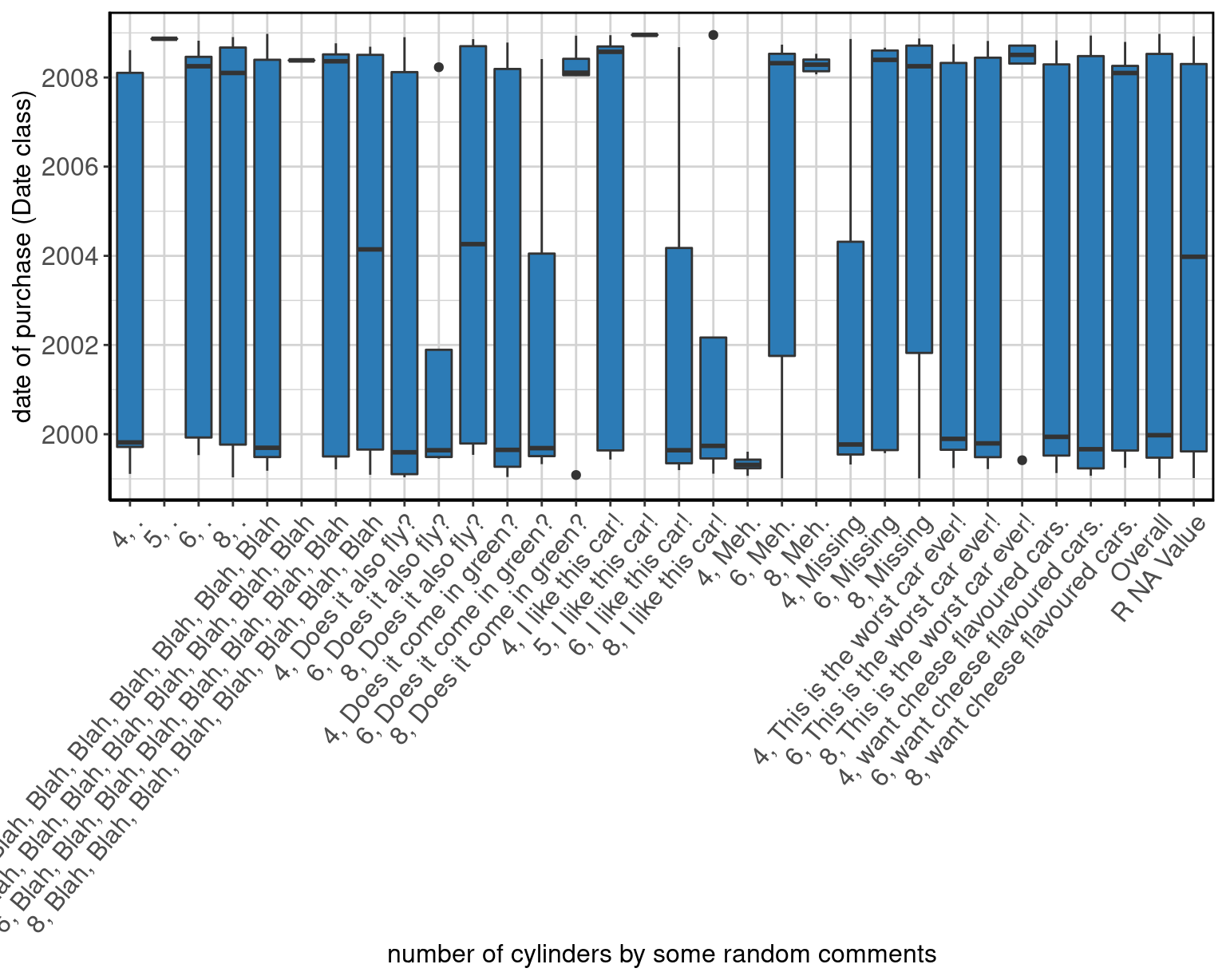
Generate a knitr friendly summary table
make_kable_output(dpByCylByCommentsSummaryExample)| number of cylinders by some random comments | Label | N | P NA | Mean | S Dev | Med | MAD | 25th P | 75th P | IQR | Min | Max |
|---|---|---|---|---|---|---|---|---|---|---|---|---|
| 4, . | date of purchase (Date class) | 5 | 0.00 | 2003-01-27 | 252.39 weeks | 1999-10-26 | 54.64 weeks | 1999-02-10 | 2008-02-08 | 469.285714 weeks | 1999-02-10 | 2008-08-12 |
| 6, . | date of purchase (Date class) | 9 | 0.00 | 2004-08-21 | 241.15 weeks | 2008-04-02 | 44.27 weeks | 1999-08-28 | 2008-06-18 | 459.571429 weeks | 1999-07-14 | 2008-10-28 |
| 8, . | date of purchase (Date class) | 10 | 9.09 | 2004-11-28 | 246.03 weeks | 2008-02-07 | 61.53 weeks | 1999-10-05 | 2008-09-06 | 465.571429 weeks | 1999-01-13 | 2008-11-27 |
| 4, Blah, Blah, Blah, Blah, Blah, Blah, Blah, Blah | date of purchase (Date class) | 9 | 0.00 | 2002-08-10 | 241.71 weeks | 1999-09-12 | 38.34 weeks | 1999-03-15 | 2008-05-25 | 479.857143 weeks | 1999-03-08 | 2008-12-23 |
| 6, Blah, Blah, Blah, Blah, Blah, Blah, Blah, Blah | date of purchase (Date class) | 7 | 12.50 | 2004-08-16 | 254.96 weeks | 2008-05-13 | 31.13 weeks | 1999-06-07 | 2008-08-02 | 477.714286 weeks | 1999-03-19 | 2008-10-07 |
| 8, Blah, Blah, Blah, Blah, Blah, Blah, Blah, Blah | date of purchase (Date class) | 4 | 0.00 | 2004-01-07 | 274.68 weeks | 2004-02-23 | 342.16 weeks | 1999-02-03 | 2008-06-12 | 488.142857 weeks | 1999-02-03 | 2008-09-09 |
| 4, Does it also fly? | date of purchase (Date class) | 5 | 0.00 | 2002-12-14 | 265.47 weeks | 1999-08-06 | 43.21 weeks | 1999-01-14 | 2008-02-14 | 474.000000 weeks | 1999-01-14 | 2008-11-26 |
| 6, Does it also fly? | date of purchase (Date class) | 4 | 42.86 | 2001-09-28 | 225.84 weeks | 1999-08-23 | 12.71 weeks | 1999-07-03 | NA | NA weeks | 1999-06-15 | 2008-03-25 |
| 8, Does it also fly? | date of purchase (Date class) | 4 | 0.00 | 2004-03-25 | 272.68 weeks | 2004-04-06 | 347.46 weeks | 1999-07-16 | 2008-08-25 | 475.428571 weeks | 1999-07-16 | 2008-11-10 |
| 4, Does it come in green? | date of purchase (Date class) | 15 | 0.00 | 2003-07-23 | 243.88 weeks | 1999-08-26 | 47.02 weeks | 1999-03-24 | 2008-02-26 | 465.857143 weeks | 1999-01-16 | 2008-10-13 |
| 6, Does it come in green? | date of purchase (Date class) | 3 | 0.00 | 2002-06-23 | 268.42 weeks | 1999-09-09 | 27.75 weeks | 1999-05-01 | 1999-09-09 | 18.714286 weeks | 1999-05-01 | 2008-05-31 |
| 8, Does it come in green? | date of purchase (Date class) | 5 | 0.00 | 2006-07-09 | 217.62 weeks | 2008-02-09 | 24.15 weeks | 1999-02-01 | 2008-06-02 | 487.000000 weeks | 1999-02-01 | 2008-12-08 |
| 4, I like this car! | date of purchase (Date class) | 8 | 11.11 | 2005-04-06 | 247.72 weeks | 2008-07-29 | 20.33 weeks | 1999-06-23 | 2008-09-23 | 482.857143 weeks | 1999-06-08 | 2008-12-12 |
| 6, I like this car! | date of purchase (Date class) | 7 | 22.22 | 2002-01-30 | 232.78 weeks | 1999-08-23 | 25.84 weeks | 1999-04-23 | 2008-09-05 | 489.000000 weeks | 1999-03-13 | 2008-09-05 |
| 8, I like this car! | date of purchase (Date class) | 4 | 0.00 | 2001-11-20 | 246.39 weeks | 1999-09-27 | 30.61 weeks | 1999-02-12 | 1999-11-28 | 41.285714 weeks | 1999-02-12 | 2008-12-14 |
| 4, Meh. | date of purchase (Date class) | 6 | 0.00 | 1999-05-01 | 9.86 weeks | 1999-04-25 | 8.47 weeks | 1999-03-26 | 1999-05-16 | 7.285714 weeks | 1999-01-25 | 1999-08-11 |
| 6, Meh. | date of purchase (Date class) | 6 | 0.00 | 2005-06-05 | 248.14 weeks | 2008-04-27 | 26.58 weeks | 1999-07-31 | 2008-05-08 | 457.714286 weeks | 1999-01-05 | 2008-09-26 |
| 8, Meh. | date of purchase (Date class) | 5 | 16.67 | 2008-04-14 | 9.80 weeks | 2008-04-15 | 11.44 weeks | 2008-02-21 | 2008-05-27 | 13.714286 weeks | 2008-01-27 | 2008-07-13 |
| 4, Missing | date of purchase (Date class) | 3 | 50.00 | 2002-08-26 | 280.92 weeks | 1999-10-09 | 34.74 weeks | 1999-10-09 | NA | NA weeks | 1999-04-28 | 2008-11-11 |
| 6, Missing | date of purchase (Date class) | 5 | 0.00 | 2004-12-23 | 255.73 weeks | 2008-05-24 | 21.18 weeks | 1999-07-30 | 2008-08-09 | 471.142857 weeks | 1999-07-30 | 2008-09-01 |
| 8, Missing | date of purchase (Date class) | 14 | 0.00 | 2005-11-13 | 226.66 weeks | 2008-04-02 | 38.55 weeks | 1999-10-04 | 2008-09-08 | 466.000000 weeks | 1999-01-04 | 2008-11-15 |
| 4, This is the worst car ever! | date of purchase (Date class) | 7 | 0.00 | 2003-05-28 | 247.48 weeks | 1999-11-24 | 50.62 weeks | 1999-06-03 | 2008-02-10 | 453.428571 weeks | 1999-03-30 | 2008-09-29 |
| 6, This is the worst car ever! | date of purchase (Date class) | 9 | 10.00 | 2002-08-03 | 237.70 weeks | 1999-10-18 | 38.34 weeks | 1999-04-20 | 2008-09-13 | 490.571429 weeks | 1999-03-22 | 2008-10-26 |
| 8, This is the worst car ever! | date of purchase (Date class) | 5 | 0.00 | 2006-09-25 | 213.60 weeks | 2008-07-04 | 16.10 weeks | 1999-06-02 | 2008-09-18 | 485.142857 weeks | 1999-06-02 | 2008-09-19 |
| 4, want cheese flavoured cars. | date of purchase (Date class) | 10 | 9.09 | 2003-02-13 | 238.91 weeks | 1999-12-10 | 57.50 weeks | 1999-06-09 | 2008-05-15 | 466.142857 weeks | 1999-02-17 | 2008-10-31 |
| 6, want cheese flavoured cars. | date of purchase (Date class) | 13 | 0.00 | 2002-04-09 | 231.98 weeks | 1999-08-31 | 36.85 weeks | 1999-03-10 | 2008-06-24 | 484.857143 weeks | 1999-01-26 | 2008-12-09 |
| 8, want cheese flavoured cars. | date of purchase (Date class) | 8 | 11.11 | 2005-01-02 | 240.53 weeks | 2008-02-06 | 44.16 weeks | 1999-05-21 | 2008-07-18 | 478.000000 weeks | 1999-04-01 | 2008-10-18 |
| Overall | date of purchase (Date class) | 213 | 8.58 | 2003-12-21 | 236.59 weeks | 1999-12-24 | 74.98 weeks | 1999-07-14 | 2008-09-01 | 476.714286 weeks | 1999-01-04 | 2008-12-23 |
| R NA Value | date of purchase (Date class) | 20 | 16.67 | 2003-12-06 | 236.95 weeks | 2003-12-24 | 337.72 weeks | 1999-08-14 | 2008-06-25 | 462.571429 weeks | 1999-01-07 | 2008-12-03 |
Generate knitr friendly output
make_complete_output(dpByCylByCommentsSummaryExample)| number of cylinders by some random comments | Label | N | P NA | Mean | S Dev | Med | MAD | 25th P | 75th P | IQR | Min | Max |
|---|---|---|---|---|---|---|---|---|---|---|---|---|
| 4, . | date of purchase (Date class) | 5 | 0.00 | 2003-01-27 | 252.39 weeks | 1999-10-26 | 54.64 weeks | 1999-02-10 | 2008-02-08 | 469.285714 weeks | 1999-02-10 | 2008-08-12 |
| 6, . | date of purchase (Date class) | 9 | 0.00 | 2004-08-21 | 241.15 weeks | 2008-04-02 | 44.27 weeks | 1999-08-28 | 2008-06-18 | 459.571429 weeks | 1999-07-14 | 2008-10-28 |
| 8, . | date of purchase (Date class) | 10 | 9.09 | 2004-11-28 | 246.03 weeks | 2008-02-07 | 61.53 weeks | 1999-10-05 | 2008-09-06 | 465.571429 weeks | 1999-01-13 | 2008-11-27 |
| 4, Blah, Blah, Blah, Blah, Blah, Blah, Blah, Blah | date of purchase (Date class) | 9 | 0.00 | 2002-08-10 | 241.71 weeks | 1999-09-12 | 38.34 weeks | 1999-03-15 | 2008-05-25 | 479.857143 weeks | 1999-03-08 | 2008-12-23 |
| 6, Blah, Blah, Blah, Blah, Blah, Blah, Blah, Blah | date of purchase (Date class) | 7 | 12.50 | 2004-08-16 | 254.96 weeks | 2008-05-13 | 31.13 weeks | 1999-06-07 | 2008-08-02 | 477.714286 weeks | 1999-03-19 | 2008-10-07 |
| 8, Blah, Blah, Blah, Blah, Blah, Blah, Blah, Blah | date of purchase (Date class) | 4 | 0.00 | 2004-01-07 | 274.68 weeks | 2004-02-23 | 342.16 weeks | 1999-02-03 | 2008-06-12 | 488.142857 weeks | 1999-02-03 | 2008-09-09 |
| 4, Does it also fly? | date of purchase (Date class) | 5 | 0.00 | 2002-12-14 | 265.47 weeks | 1999-08-06 | 43.21 weeks | 1999-01-14 | 2008-02-14 | 474.000000 weeks | 1999-01-14 | 2008-11-26 |
| 6, Does it also fly? | date of purchase (Date class) | 4 | 42.86 | 2001-09-28 | 225.84 weeks | 1999-08-23 | 12.71 weeks | 1999-07-03 | NA | NA weeks | 1999-06-15 | 2008-03-25 |
| 8, Does it also fly? | date of purchase (Date class) | 4 | 0.00 | 2004-03-25 | 272.68 weeks | 2004-04-06 | 347.46 weeks | 1999-07-16 | 2008-08-25 | 475.428571 weeks | 1999-07-16 | 2008-11-10 |
| 4, Does it come in green? | date of purchase (Date class) | 15 | 0.00 | 2003-07-23 | 243.88 weeks | 1999-08-26 | 47.02 weeks | 1999-03-24 | 2008-02-26 | 465.857143 weeks | 1999-01-16 | 2008-10-13 |
| 6, Does it come in green? | date of purchase (Date class) | 3 | 0.00 | 2002-06-23 | 268.42 weeks | 1999-09-09 | 27.75 weeks | 1999-05-01 | 1999-09-09 | 18.714286 weeks | 1999-05-01 | 2008-05-31 |
| 8, Does it come in green? | date of purchase (Date class) | 5 | 0.00 | 2006-07-09 | 217.62 weeks | 2008-02-09 | 24.15 weeks | 1999-02-01 | 2008-06-02 | 487.000000 weeks | 1999-02-01 | 2008-12-08 |
| 4, I like this car! | date of purchase (Date class) | 8 | 11.11 | 2005-04-06 | 247.72 weeks | 2008-07-29 | 20.33 weeks | 1999-06-23 | 2008-09-23 | 482.857143 weeks | 1999-06-08 | 2008-12-12 |
| 6, I like this car! | date of purchase (Date class) | 7 | 22.22 | 2002-01-30 | 232.78 weeks | 1999-08-23 | 25.84 weeks | 1999-04-23 | 2008-09-05 | 489.000000 weeks | 1999-03-13 | 2008-09-05 |
| 8, I like this car! | date of purchase (Date class) | 4 | 0.00 | 2001-11-20 | 246.39 weeks | 1999-09-27 | 30.61 weeks | 1999-02-12 | 1999-11-28 | 41.285714 weeks | 1999-02-12 | 2008-12-14 |
| 4, Meh. | date of purchase (Date class) | 6 | 0.00 | 1999-05-01 | 9.86 weeks | 1999-04-25 | 8.47 weeks | 1999-03-26 | 1999-05-16 | 7.285714 weeks | 1999-01-25 | 1999-08-11 |
| 6, Meh. | date of purchase (Date class) | 6 | 0.00 | 2005-06-05 | 248.14 weeks | 2008-04-27 | 26.58 weeks | 1999-07-31 | 2008-05-08 | 457.714286 weeks | 1999-01-05 | 2008-09-26 |
| 8, Meh. | date of purchase (Date class) | 5 | 16.67 | 2008-04-14 | 9.80 weeks | 2008-04-15 | 11.44 weeks | 2008-02-21 | 2008-05-27 | 13.714286 weeks | 2008-01-27 | 2008-07-13 |
| 4, Missing | date of purchase (Date class) | 3 | 50.00 | 2002-08-26 | 280.92 weeks | 1999-10-09 | 34.74 weeks | 1999-10-09 | NA | NA weeks | 1999-04-28 | 2008-11-11 |
| 6, Missing | date of purchase (Date class) | 5 | 0.00 | 2004-12-23 | 255.73 weeks | 2008-05-24 | 21.18 weeks | 1999-07-30 | 2008-08-09 | 471.142857 weeks | 1999-07-30 | 2008-09-01 |
| 8, Missing | date of purchase (Date class) | 14 | 0.00 | 2005-11-13 | 226.66 weeks | 2008-04-02 | 38.55 weeks | 1999-10-04 | 2008-09-08 | 466.000000 weeks | 1999-01-04 | 2008-11-15 |
| 4, This is the worst car ever! | date of purchase (Date class) | 7 | 0.00 | 2003-05-28 | 247.48 weeks | 1999-11-24 | 50.62 weeks | 1999-06-03 | 2008-02-10 | 453.428571 weeks | 1999-03-30 | 2008-09-29 |
| 6, This is the worst car ever! | date of purchase (Date class) | 9 | 10.00 | 2002-08-03 | 237.70 weeks | 1999-10-18 | 38.34 weeks | 1999-04-20 | 2008-09-13 | 490.571429 weeks | 1999-03-22 | 2008-10-26 |
| 8, This is the worst car ever! | date of purchase (Date class) | 5 | 0.00 | 2006-09-25 | 213.60 weeks | 2008-07-04 | 16.10 weeks | 1999-06-02 | 2008-09-18 | 485.142857 weeks | 1999-06-02 | 2008-09-19 |
| 4, want cheese flavoured cars. | date of purchase (Date class) | 10 | 9.09 | 2003-02-13 | 238.91 weeks | 1999-12-10 | 57.50 weeks | 1999-06-09 | 2008-05-15 | 466.142857 weeks | 1999-02-17 | 2008-10-31 |
| 6, want cheese flavoured cars. | date of purchase (Date class) | 13 | 0.00 | 2002-04-09 | 231.98 weeks | 1999-08-31 | 36.85 weeks | 1999-03-10 | 2008-06-24 | 484.857143 weeks | 1999-01-26 | 2008-12-09 |
| 8, want cheese flavoured cars. | date of purchase (Date class) | 8 | 11.11 | 2005-01-02 | 240.53 weeks | 2008-02-06 | 44.16 weeks | 1999-05-21 | 2008-07-18 | 478.000000 weeks | 1999-04-01 | 2008-10-18 |
| Overall | date of purchase (Date class) | 213 | 8.58 | 2003-12-21 | 236.59 weeks | 1999-12-24 | 74.98 weeks | 1999-07-14 | 2008-09-01 | 476.714286 weeks | 1999-01-04 | 2008-12-23 |
| R NA Value | date of purchase (Date class) | 20 | 16.67 | 2003-12-06 | 236.95 weeks | 2003-12-24 | 337.72 weeks | 1999-08-14 | 2008-06-25 | 462.571429 weeks | 1999-01-07 | 2008-12-03 |

Figure 9: Stacked barplot of date of purchase (Date class) by number of cylinders by some random comments.
POSIXlt Date
For a date variable x, we need to specify x, the data, and difftime_units.
dpltSummaryExample <- data_summary(x = "dplt", data = mpg, difftime_units = "weeks")Show method to output table and plot
show(dpltSummaryExample)## Label N P NA Mean S Dev
## 1 date of purchase (POSIXlt class) 234 8.55 2003-11-15 13:01:05 234.3 weeks
## Med MAD 25th P 75th P
## 1 1999-12-16 04:23:30 67.67 weeks 1999-07-17 09:42:00 2008-07-23 15:02:51
## IQR Min Max
## 1 470.6033 weeks 1999-01-04 04:59:00 2008-12-23 01:06:02
Output the summary table
data_summary_table(dpltSummaryExample)## Label N P NA Mean S Dev
## 1 date of purchase (POSIXlt class) 234 8.55 2003-11-15 13:01:05 234.3 weeks
## Med MAD 25th P 75th P
## 1 1999-12-16 04:23:30 67.67 weeks 1999-07-17 09:42:00 2008-07-23 15:02:51
## IQR Min Max
## 1 470.6033 weeks 1999-01-04 04:59:00 2008-12-23 01:06:02Output the plot
data_summary_plot(dpltSummaryExample)
Generate knitr friendly summary table
make_kable_output(dpltSummaryExample)| Label | N | P NA | Mean | S Dev | Med | MAD | 25th P | 75th P | IQR | Min | Max | |
|---|---|---|---|---|---|---|---|---|---|---|---|---|
| date of purchase (POSIXlt class) | 234 | 8.55 | 2003-11-15 13:01:05 | 234.3 weeks | 1999-12-16 04:23:30 | 67.67 weeks | 1999-07-17 09:42:00 | 2008-07-23 15:02:51 | 470.6033 weeks | 1999-01-04 04:59:00 | 2008-12-23 01:06:02 |
Generate knitr friendly output
make_complete_output(dpltSummaryExample)| Label | N | P NA | Mean | S Dev | Med | MAD | 25th P | 75th P | IQR | Min | Max | |
|---|---|---|---|---|---|---|---|---|---|---|---|---|
| date of purchase (POSIXlt class) | 234 | 8.55 | 2003-11-15 13:01:05 | 234.3 weeks | 1999-12-16 04:23:30 | 67.67 weeks | 1999-07-17 09:42:00 | 2008-07-23 15:02:51 | 470.6033 weeks | 1999-01-04 04:59:00 | 2008-12-23 01:06:02 |

Figure 10: Stacked barplot of date of purchase (Date class).
POSIXlt Date By
For a date variable with by, we need to specify x, a by variable, the data, and difftime_units.
dpltByCylSummaryExample <- data_summary(x = "dplt", by = "cyl", data = mpg, difftime_units = "weeks")Show method to output table and plot
show(dpltByCylSummaryExample)## number of cylinders Label N P NA
## 1 4 date of purchase (POSIXlt class) 81 8.64
## 2 5 date of purchase (POSIXlt class) 4 0.00
## 3 6 date of purchase (POSIXlt class) 79 7.59
## 4 8 date of purchase (POSIXlt class) 70 10.00
## 5 Overall date of purchase (POSIXlt class) 234 8.55
## Mean S Dev Med MAD
## 1 2003-06-07 08:46:09 230.17 weeks 1999-11-21 23:21:30 44.34 weeks
## 2 2008-06-18 21:25:47 17.06 weeks 2008-06-19 01:08:01 21.71 weeks
## 3 2002-12-18 08:32:02 231.02 weeks 1999-09-23 07:05:00 38.02 weeks
## 4 2005-02-25 06:40:15 229.55 weeks 2008-02-28 14:28:40 52.72 weeks
## 5 2003-11-15 13:01:05 234.30 weeks 1999-12-16 04:23:30 67.67 weeks
## 25th P 75th P IQR Min
## 1 1999-08-17 06:59:00 2008-07-19 05:48:36 465.56444 weeks 1999-02-06 23:51:00
## 2 2008-02-24 08:01:04 2008-09-16 22:32:21 29.37215 weeks 2008-02-24 08:01:04
## 3 1999-06-01 04:12:00 2008-06-29 23:50:43 473.83122 weeks 1999-02-02 05:57:00
## 4 1999-08-02 23:23:00 2008-08-16 20:36:23 471.69776 weeks 1999-01-04 04:59:00
## 5 1999-07-17 09:42:00 2008-07-23 15:02:51 470.60326 weeks 1999-01-04 04:59:00
## Max
## 1 2008-12-06 16:25:11
## 2 2008-10-12 03:26:02
## 3 2008-12-23 01:06:02
## 4 2008-12-15 06:26:36
## 5 2008-12-23 01:06:02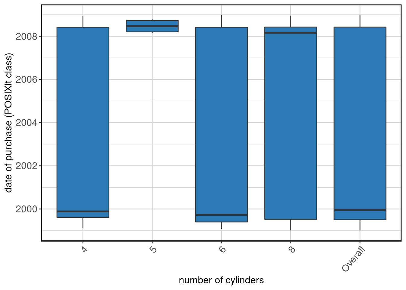
Output the summary table
data_summary_table(dpltByCylSummaryExample)## number of cylinders Label N P NA
## 1 4 date of purchase (POSIXlt class) 81 8.64
## 2 5 date of purchase (POSIXlt class) 4 0.00
## 3 6 date of purchase (POSIXlt class) 79 7.59
## 4 8 date of purchase (POSIXlt class) 70 10.00
## 5 Overall date of purchase (POSIXlt class) 234 8.55
## Mean S Dev Med MAD
## 1 2003-06-07 08:46:09 230.17 weeks 1999-11-21 23:21:30 44.34 weeks
## 2 2008-06-18 21:25:47 17.06 weeks 2008-06-19 01:08:01 21.71 weeks
## 3 2002-12-18 08:32:02 231.02 weeks 1999-09-23 07:05:00 38.02 weeks
## 4 2005-02-25 06:40:15 229.55 weeks 2008-02-28 14:28:40 52.72 weeks
## 5 2003-11-15 13:01:05 234.30 weeks 1999-12-16 04:23:30 67.67 weeks
## 25th P 75th P IQR Min
## 1 1999-08-17 06:59:00 2008-07-19 05:48:36 465.56444 weeks 1999-02-06 23:51:00
## 2 2008-02-24 08:01:04 2008-09-16 22:32:21 29.37215 weeks 2008-02-24 08:01:04
## 3 1999-06-01 04:12:00 2008-06-29 23:50:43 473.83122 weeks 1999-02-02 05:57:00
## 4 1999-08-02 23:23:00 2008-08-16 20:36:23 471.69776 weeks 1999-01-04 04:59:00
## 5 1999-07-17 09:42:00 2008-07-23 15:02:51 470.60326 weeks 1999-01-04 04:59:00
## Max
## 1 2008-12-06 16:25:11
## 2 2008-10-12 03:26:02
## 3 2008-12-23 01:06:02
## 4 2008-12-15 06:26:36
## 5 2008-12-23 01:06:02Output the plot
data_summary_plot(dpltByCylSummaryExample)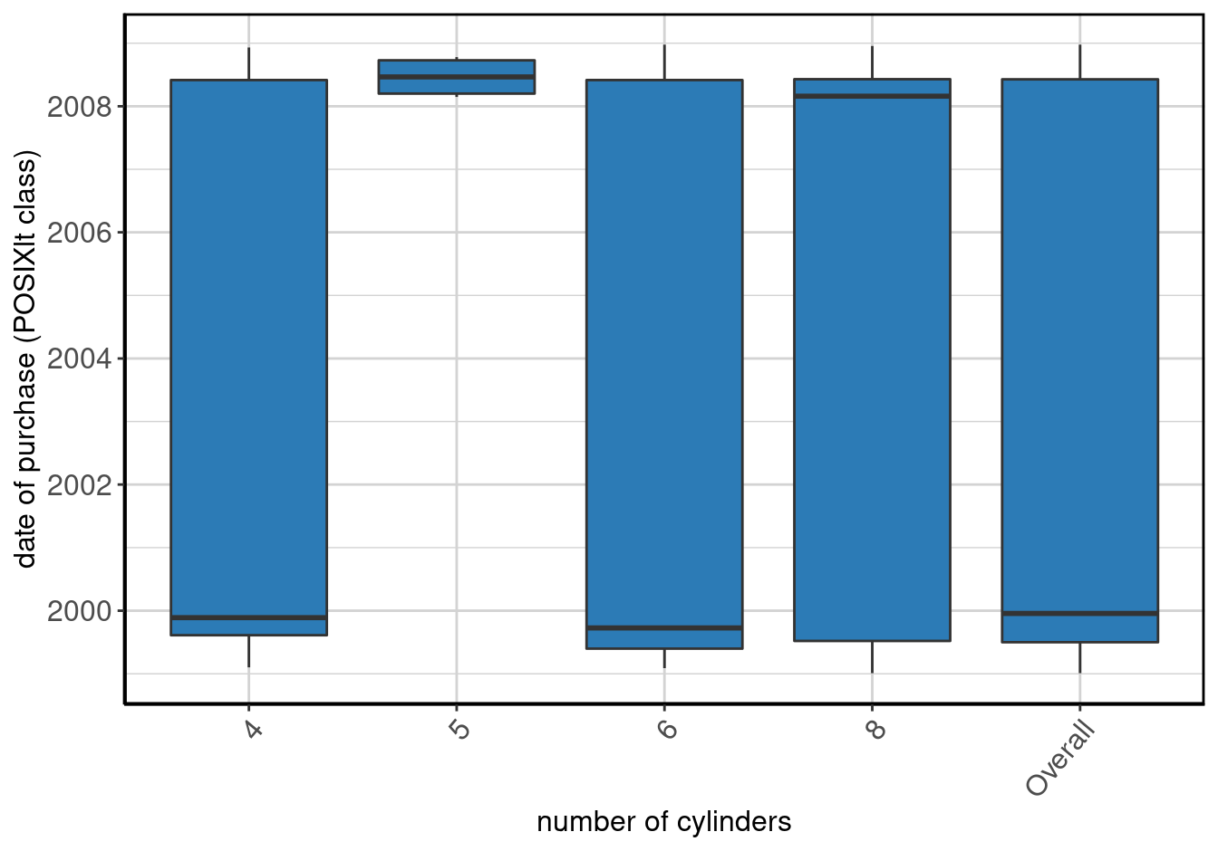
Generate a knitr friendly summary table
make_kable_output(dpltByCylSummaryExample)| number of cylinders | Label | N | P NA | Mean | S Dev | Med | MAD | 25th P | 75th P | IQR | Min | Max |
|---|---|---|---|---|---|---|---|---|---|---|---|---|
| 4 | date of purchase (POSIXlt class) | 81 | 8.64 | 2003-06-07 08:46:09 | 230.17 weeks | 1999-11-21 23:21:30 | 44.34 weeks | 1999-08-17 06:59:00 | 2008-07-19 05:48:36 | 465.56444 weeks | 1999-02-06 23:51:00 | 2008-12-06 16:25:11 |
| 5 | date of purchase (POSIXlt class) | 4 | 0.00 | 2008-06-18 21:25:47 | 17.06 weeks | 2008-06-19 01:08:01 | 21.71 weeks | 2008-02-24 08:01:04 | 2008-09-16 22:32:21 | 29.37215 weeks | 2008-02-24 08:01:04 | 2008-10-12 03:26:02 |
| 6 | date of purchase (POSIXlt class) | 79 | 7.59 | 2002-12-18 08:32:02 | 231.02 weeks | 1999-09-23 07:05:00 | 38.02 weeks | 1999-06-01 04:12:00 | 2008-06-29 23:50:43 | 473.83122 weeks | 1999-02-02 05:57:00 | 2008-12-23 01:06:02 |
| 8 | date of purchase (POSIXlt class) | 70 | 10.00 | 2005-02-25 06:40:15 | 229.55 weeks | 2008-02-28 14:28:40 | 52.72 weeks | 1999-08-02 23:23:00 | 2008-08-16 20:36:23 | 471.69776 weeks | 1999-01-04 04:59:00 | 2008-12-15 06:26:36 |
| Overall | date of purchase (POSIXlt class) | 234 | 8.55 | 2003-11-15 13:01:05 | 234.30 weeks | 1999-12-16 04:23:30 | 67.67 weeks | 1999-07-17 09:42:00 | 2008-07-23 15:02:51 | 470.60326 weeks | 1999-01-04 04:59:00 | 2008-12-23 01:06:02 |
Generate knitr friendly output
make_complete_output(dpltByCylSummaryExample)| number of cylinders | Label | N | P NA | Mean | S Dev | Med | MAD | 25th P | 75th P | IQR | Min | Max |
|---|---|---|---|---|---|---|---|---|---|---|---|---|
| 4 | date of purchase (POSIXlt class) | 81 | 8.64 | 2003-06-07 08:46:09 | 230.17 weeks | 1999-11-21 23:21:30 | 44.34 weeks | 1999-08-17 06:59:00 | 2008-07-19 05:48:36 | 465.56444 weeks | 1999-02-06 23:51:00 | 2008-12-06 16:25:11 |
| 5 | date of purchase (POSIXlt class) | 4 | 0.00 | 2008-06-18 21:25:47 | 17.06 weeks | 2008-06-19 01:08:01 | 21.71 weeks | 2008-02-24 08:01:04 | 2008-09-16 22:32:21 | 29.37215 weeks | 2008-02-24 08:01:04 | 2008-10-12 03:26:02 |
| 6 | date of purchase (POSIXlt class) | 79 | 7.59 | 2002-12-18 08:32:02 | 231.02 weeks | 1999-09-23 07:05:00 | 38.02 weeks | 1999-06-01 04:12:00 | 2008-06-29 23:50:43 | 473.83122 weeks | 1999-02-02 05:57:00 | 2008-12-23 01:06:02 |
| 8 | date of purchase (POSIXlt class) | 70 | 10.00 | 2005-02-25 06:40:15 | 229.55 weeks | 2008-02-28 14:28:40 | 52.72 weeks | 1999-08-02 23:23:00 | 2008-08-16 20:36:23 | 471.69776 weeks | 1999-01-04 04:59:00 | 2008-12-15 06:26:36 |
| Overall | date of purchase (POSIXlt class) | 234 | 8.55 | 2003-11-15 13:01:05 | 234.30 weeks | 1999-12-16 04:23:30 | 67.67 weeks | 1999-07-17 09:42:00 | 2008-07-23 15:02:51 | 470.60326 weeks | 1999-01-04 04:59:00 | 2008-12-23 01:06:02 |

Figure 11: Stacked barplot of date of purchase (Date class) by number of cylinders.
POSIXlt Date By By
For a date variable with two or more by variables, we need to specify x, the by variables as a character string, the data, and difftime_units.
dpltByCylByCommentsSummaryExample <- data_summary(x = "dplt", by = c("cyl", "comments"), data = mpg, difftime_units = "weeks")Show method to output table and plot
show(dpltByCylByCommentsSummaryExample)## number of cylinders by some random comments
## 1 4, .
## 2 6, .
## 3 8, .
## 4 4, Blah, Blah, Blah, Blah, Blah, Blah, Blah, Blah
## 5 6, Blah, Blah, Blah, Blah, Blah, Blah, Blah, Blah
## 6 8, Blah, Blah, Blah, Blah, Blah, Blah, Blah, Blah
## 7 4, Does it also fly?
## 8 6, Does it also fly?
## 9 8, Does it also fly?
## 10 4, Does it come in green?
## 11 6, Does it come in green?
## 12 8, Does it come in green?
## 13 4, I like this car!
## 14 6, I like this car!
## 15 8, I like this car!
## 16 4, Meh.
## 17 6, Meh.
## 18 8, Meh.
## 19 4, Missing
## 20 6, Missing
## 21 8, Missing
## 22 4, This is the worst car ever!
## 23 6, This is the worst car ever!
## 24 8, This is the worst car ever!
## 25 4, want cheese flavoured cars.
## 26 6, want cheese flavoured cars.
## 27 8, want cheese flavoured cars.
## 28 Overall
## 29 R NA Value
## Label N P NA Mean S Dev
## 1 date of purchase (POSIXlt class) 5 0.00 2002-12-26 13:38:31 260.08 weeks
## 2 date of purchase (POSIXlt class) 9 11.11 2003-12-31 07:58:18 247.12 weeks
## 3 date of purchase (POSIXlt class) 11 0.00 2004-05-29 01:24:54 245.48 weeks
## 4 date of purchase (POSIXlt class) 9 0.00 2002-06-23 09:51:45 223.34 weeks
## 5 date of purchase (POSIXlt class) 8 12.50 2004-07-24 20:46:13 261.15 weeks
## 6 date of purchase (POSIXlt class) 4 50.00 2008-05-14 05:42:44 2.05 weeks
## 7 date of purchase (POSIXlt class) 5 0.00 2003-03-07 13:02:00 254.76 weeks
## 8 date of purchase (POSIXlt class) 7 14.29 2000-12-31 00:40:43 201.17 weeks
## 9 date of purchase (POSIXlt class) 4 0.00 2003-12-13 22:25:46 278.25 weeks
## 10 date of purchase (POSIXlt class) 15 6.67 2003-06-16 06:56:21 236.42 weeks
## 11 date of purchase (POSIXlt class) 3 0.00 2002-06-30 08:12:42 270.33 weeks
## 12 date of purchase (POSIXlt class) 5 0.00 2006-10-07 03:49:16 212.99 weeks
## 13 date of purchase (POSIXlt class) 10 0.00 2004-11-13 07:26:51 239.01 weeks
## 14 date of purchase (POSIXlt class) 9 0.00 2001-07-09 07:24:32 208.13 weeks
## 15 date of purchase (POSIXlt class) 4 0.00 2001-07-01 15:33:59 239.79 weeks
## 16 date of purchase (POSIXlt class) 6 0.00 1999-08-25 12:01:40 9.25 weeks
## 17 date of purchase (POSIXlt class) 6 0.00 2005-06-27 05:16:57 237.83 weeks
## 18 date of purchase (POSIXlt class) 6 16.67 2008-04-25 09:42:01 7.88 weeks
## 19 date of purchase (POSIXlt class) 6 33.33 2004-02-24 10:35:52 267.91 weeks
## 20 date of purchase (POSIXlt class) 5 0.00 2004-10-25 01:13:27 267.95 weeks
## 21 date of purchase (POSIXlt class) 14 14.29 2006-04-18 06:42:10 206.29 weeks
## 22 date of purchase (POSIXlt class) 7 0.00 2003-04-05 22:54:10 245.37 weeks
## 23 date of purchase (POSIXlt class) 10 10.00 2002-08-17 05:20:29 241.20 weeks
## 24 date of purchase (POSIXlt class) 5 0.00 2006-08-16 08:39:48 207.93 weeks
## 25 date of purchase (POSIXlt class) 11 36.36 2004-09-23 18:01:28 249.43 weeks
## 26 date of purchase (POSIXlt class) 13 7.69 2001-10-13 08:39:46 206.72 weeks
## 27 date of purchase (POSIXlt class) 9 22.22 2004-09-01 03:43:02 260.61 weeks
## 28 date of purchase (POSIXlt class) 234 8.55 2003-11-15 13:01:05 234.30 weeks
## 29 date of purchase (POSIXlt class) 24 4.17 2003-05-14 05:30:18 237.27 weeks
## Med MAD 25th P 75th P
## 1 1999-06-24 09:05:00 17.72 weeks 1999-04-01 16:49:00 2008-05-04 13:32:00
## 2 2004-01-11 07:48:34 340.15 weeks 1999-06-21 14:04:00 2008-05-07 11:07:04
## 3 2008-01-08 08:48:50 69.28 weeks 1999-06-17 19:51:00 2008-06-16 10:15:19
## 4 1999-11-10 03:37:00 28.85 weeks 1999-06-26 22:47:00 2008-01-01 21:17:41
## 5 2008-04-06 04:33:44 50.36 weeks 1999-03-18 09:04:00 2008-09-11 11:16:05
## 6 2008-05-14 05:42:44 2.15 weeks 2008-05-04 02:11:56 <NA>
## 7 1999-12-03 14:02:00 46.46 weeks 1999-04-28 06:00:00 2008-02-04 15:09:51
## 8 1999-05-30 16:24:30 12.40 weeks 1999-05-05 05:29:00 1999-10-26 17:15:00
## 9 2003-11-02 13:02:39 348.06 weeks 1999-04-03 04:24:00 2008-04-01 21:16:18
## 10 1999-11-24 15:28:30 39.39 weeks 1999-09-02 05:35:00 2008-07-23 15:02:51
## 11 1999-08-29 03:43:00 23.66 weeks 1999-05-09 11:09:00 1999-08-29 03:43:00
## 12 2008-04-16 09:43:47 42.60 weeks 1999-06-27 01:00:00 2008-11-03 12:36:31
## 13 2008-02-20 02:59:31 43.53 weeks 1999-07-19 01:45:00 2008-06-05 23:16:30
## 14 1999-09-01 02:08:00 21.11 weeks 1999-05-20 04:21:00 1999-10-17 19:26:00
## 15 1999-03-21 09:08:00 2.24 weeks 1999-03-03 10:20:00 1999-03-24 14:33:00
## 16 1999-08-28 23:33:00 6.94 weeks 1999-08-04 16:17:00 1999-09-09 16:07:00
## 17 2008-05-07 15:52:30 12.18 weeks 1999-10-01 21:39:00 2008-06-02 21:26:13
## 18 2008-04-22 03:39:45 4.67 weeks 2008-03-31 02:48:18 2008-05-06 10:35:30
## 19 2004-02-24 04:39:56 343.94 weeks 1999-09-16 12:56:00 2008-08-08 07:13:36
## 20 2008-07-21 13:26:31 2.15 weeks 1999-02-23 01:03:00 2008-07-24 03:53:54
## 21 2008-05-04 22:11:45 28.88 weeks 2008-01-15 10:13:33 2008-10-14 02:45:41
## 22 1999-10-03 19:59:00 40.91 weeks 1999-04-01 16:56:00 2008-02-06 14:44:36
## 23 1999-09-23 07:05:00 31.28 weeks 1999-04-28 14:16:00 2008-11-24 04:28:26
## 24 2008-05-16 14:45:50 18.25 weeks 1999-07-03 07:38:00 2008-06-23 13:12:36
## 25 2008-02-20 02:52:27 51.90 weeks 1999-09-24 22:41:00 <NA>
## 26 1999-09-17 06:54:30 16.31 weeks 1999-07-02 01:34:00 2008-04-01 21:06:18
## 27 2008-01-19 02:34:35 67.07 weeks 1999-06-20 13:17:00 2008-11-30 18:38:11
## 28 1999-12-16 04:23:30 67.67 weeks 1999-07-17 09:42:00 2008-07-23 15:02:51
## 29 1999-12-02 03:54:00 64.95 weeks 1999-04-07 11:51:00 2008-05-14 10:48:26
## IQR Min Max
## 1 474.409028 weeks 1999-04-01 16:49:00 2008-07-19 05:48:36
## 2 463.268161 weeks 1999-06-01 04:12:00 2008-11-12 17:56:39
## 3 469.514317 weeks 1999-01-31 21:39:00 2008-11-30 10:47:06
## 4 444.419711 weeks 1999-02-06 23:51:00 2008-06-22 01:19:06
## 5 495.013104 weeks 1999-02-02 05:57:00 2008-11-29 23:22:31
## 6 NA weeks 2008-05-04 02:11:56 2008-05-24 09:13:33
## 7 457.768834 weeks 1999-04-28 06:00:00 2008-12-06 16:25:11
## 8 24.927183 weeks 1999-02-28 00:08:00 2008-11-08 20:23:21
## 9 469.528998 weeks 1999-04-03 04:24:00 2008-11-15 11:13:47
## 10 463.913477 weeks 1999-05-08 11:54:00 2008-10-21 20:32:53
## 11 15.955754 weeks 1999-05-09 11:09:00 2008-06-22 09:46:07
## 12 488.211956 weeks 1999-06-27 01:00:00 2008-12-13 19:57:34
## 13 463.556696 weeks 1999-05-25 08:23:00 2008-09-27 22:41:44
## 14 21.518353 weeks 1999-04-06 04:38:00 2008-12-23 01:06:02
## 15 3.025099 weeks 1999-03-03 10:20:00 2008-05-23 09:39:59
## 16 5.141865 weeks 1999-05-07 20:04:00 1999-11-12 08:41:00
## 17 452.427303 weeks 1999-06-17 18:37:00 2008-07-19 02:28:08
## 18 5.189206 weeks 2008-02-19 04:00:08 2008-07-18 03:26:27
## 19 464.108889 weeks 1999-09-12 01:50:00 2008-08-08 07:13:36
## 20 491.302669 weeks 1999-02-23 01:03:00 2008-07-31 16:39:54
## 21 38.955569 weeks 1999-08-02 23:23:00 2008-12-15 06:26:36
## 22 461.844107 weeks 1999-03-24 16:04:00 2008-06-16 19:57:55
## 23 499.655995 weeks 1999-02-22 04:55:00 2008-11-29 02:51:30
## 24 468.318909 weeks 1999-07-03 07:38:00 2008-08-16 20:36:23
## 25 NA weeks 1999-07-17 09:42:00 2008-10-22 03:49:26
## 26 456.687728 weeks 1999-02-02 06:27:00 2008-06-29 23:50:43
## 27 493.031863 weeks 1999-01-06 16:15:00 2008-11-30 18:38:11
## 28 470.603259 weeks 1999-01-04 04:59:00 2008-12-23 01:06:02
## 29 474.993793 weeks 1999-01-04 04:59:00 2008-10-23 18:14:24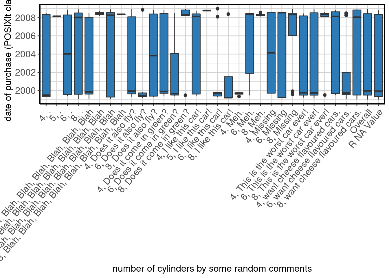
Output the summary table
data_summary_table(dpltByCylByCommentsSummaryExample)## number of cylinders by some random comments
## 1 4, .
## 2 6, .
## 3 8, .
## 4 4, Blah, Blah, Blah, Blah, Blah, Blah, Blah, Blah
## 5 6, Blah, Blah, Blah, Blah, Blah, Blah, Blah, Blah
## 6 8, Blah, Blah, Blah, Blah, Blah, Blah, Blah, Blah
## 7 4, Does it also fly?
## 8 6, Does it also fly?
## 9 8, Does it also fly?
## 10 4, Does it come in green?
## 11 6, Does it come in green?
## 12 8, Does it come in green?
## 13 4, I like this car!
## 14 6, I like this car!
## 15 8, I like this car!
## 16 4, Meh.
## 17 6, Meh.
## 18 8, Meh.
## 19 4, Missing
## 20 6, Missing
## 21 8, Missing
## 22 4, This is the worst car ever!
## 23 6, This is the worst car ever!
## 24 8, This is the worst car ever!
## 25 4, want cheese flavoured cars.
## 26 6, want cheese flavoured cars.
## 27 8, want cheese flavoured cars.
## 28 Overall
## 29 R NA Value
## Label N P NA Mean S Dev
## 1 date of purchase (POSIXlt class) 5 0.00 2002-12-26 13:38:31 260.08 weeks
## 2 date of purchase (POSIXlt class) 9 11.11 2003-12-31 07:58:18 247.12 weeks
## 3 date of purchase (POSIXlt class) 11 0.00 2004-05-29 01:24:54 245.48 weeks
## 4 date of purchase (POSIXlt class) 9 0.00 2002-06-23 09:51:45 223.34 weeks
## 5 date of purchase (POSIXlt class) 8 12.50 2004-07-24 20:46:13 261.15 weeks
## 6 date of purchase (POSIXlt class) 4 50.00 2008-05-14 05:42:44 2.05 weeks
## 7 date of purchase (POSIXlt class) 5 0.00 2003-03-07 13:02:00 254.76 weeks
## 8 date of purchase (POSIXlt class) 7 14.29 2000-12-31 00:40:43 201.17 weeks
## 9 date of purchase (POSIXlt class) 4 0.00 2003-12-13 22:25:46 278.25 weeks
## 10 date of purchase (POSIXlt class) 15 6.67 2003-06-16 06:56:21 236.42 weeks
## 11 date of purchase (POSIXlt class) 3 0.00 2002-06-30 08:12:42 270.33 weeks
## 12 date of purchase (POSIXlt class) 5 0.00 2006-10-07 03:49:16 212.99 weeks
## 13 date of purchase (POSIXlt class) 10 0.00 2004-11-13 07:26:51 239.01 weeks
## 14 date of purchase (POSIXlt class) 9 0.00 2001-07-09 07:24:32 208.13 weeks
## 15 date of purchase (POSIXlt class) 4 0.00 2001-07-01 15:33:59 239.79 weeks
## 16 date of purchase (POSIXlt class) 6 0.00 1999-08-25 12:01:40 9.25 weeks
## 17 date of purchase (POSIXlt class) 6 0.00 2005-06-27 05:16:57 237.83 weeks
## 18 date of purchase (POSIXlt class) 6 16.67 2008-04-25 09:42:01 7.88 weeks
## 19 date of purchase (POSIXlt class) 6 33.33 2004-02-24 10:35:52 267.91 weeks
## 20 date of purchase (POSIXlt class) 5 0.00 2004-10-25 01:13:27 267.95 weeks
## 21 date of purchase (POSIXlt class) 14 14.29 2006-04-18 06:42:10 206.29 weeks
## 22 date of purchase (POSIXlt class) 7 0.00 2003-04-05 22:54:10 245.37 weeks
## 23 date of purchase (POSIXlt class) 10 10.00 2002-08-17 05:20:29 241.20 weeks
## 24 date of purchase (POSIXlt class) 5 0.00 2006-08-16 08:39:48 207.93 weeks
## 25 date of purchase (POSIXlt class) 11 36.36 2004-09-23 18:01:28 249.43 weeks
## 26 date of purchase (POSIXlt class) 13 7.69 2001-10-13 08:39:46 206.72 weeks
## 27 date of purchase (POSIXlt class) 9 22.22 2004-09-01 03:43:02 260.61 weeks
## 28 date of purchase (POSIXlt class) 234 8.55 2003-11-15 13:01:05 234.30 weeks
## 29 date of purchase (POSIXlt class) 24 4.17 2003-05-14 05:30:18 237.27 weeks
## Med MAD 25th P 75th P
## 1 1999-06-24 09:05:00 17.72 weeks 1999-04-01 16:49:00 2008-05-04 13:32:00
## 2 2004-01-11 07:48:34 340.15 weeks 1999-06-21 14:04:00 2008-05-07 11:07:04
## 3 2008-01-08 08:48:50 69.28 weeks 1999-06-17 19:51:00 2008-06-16 10:15:19
## 4 1999-11-10 03:37:00 28.85 weeks 1999-06-26 22:47:00 2008-01-01 21:17:41
## 5 2008-04-06 04:33:44 50.36 weeks 1999-03-18 09:04:00 2008-09-11 11:16:05
## 6 2008-05-14 05:42:44 2.15 weeks 2008-05-04 02:11:56 <NA>
## 7 1999-12-03 14:02:00 46.46 weeks 1999-04-28 06:00:00 2008-02-04 15:09:51
## 8 1999-05-30 16:24:30 12.40 weeks 1999-05-05 05:29:00 1999-10-26 17:15:00
## 9 2003-11-02 13:02:39 348.06 weeks 1999-04-03 04:24:00 2008-04-01 21:16:18
## 10 1999-11-24 15:28:30 39.39 weeks 1999-09-02 05:35:00 2008-07-23 15:02:51
## 11 1999-08-29 03:43:00 23.66 weeks 1999-05-09 11:09:00 1999-08-29 03:43:00
## 12 2008-04-16 09:43:47 42.60 weeks 1999-06-27 01:00:00 2008-11-03 12:36:31
## 13 2008-02-20 02:59:31 43.53 weeks 1999-07-19 01:45:00 2008-06-05 23:16:30
## 14 1999-09-01 02:08:00 21.11 weeks 1999-05-20 04:21:00 1999-10-17 19:26:00
## 15 1999-03-21 09:08:00 2.24 weeks 1999-03-03 10:20:00 1999-03-24 14:33:00
## 16 1999-08-28 23:33:00 6.94 weeks 1999-08-04 16:17:00 1999-09-09 16:07:00
## 17 2008-05-07 15:52:30 12.18 weeks 1999-10-01 21:39:00 2008-06-02 21:26:13
## 18 2008-04-22 03:39:45 4.67 weeks 2008-03-31 02:48:18 2008-05-06 10:35:30
## 19 2004-02-24 04:39:56 343.94 weeks 1999-09-16 12:56:00 2008-08-08 07:13:36
## 20 2008-07-21 13:26:31 2.15 weeks 1999-02-23 01:03:00 2008-07-24 03:53:54
## 21 2008-05-04 22:11:45 28.88 weeks 2008-01-15 10:13:33 2008-10-14 02:45:41
## 22 1999-10-03 19:59:00 40.91 weeks 1999-04-01 16:56:00 2008-02-06 14:44:36
## 23 1999-09-23 07:05:00 31.28 weeks 1999-04-28 14:16:00 2008-11-24 04:28:26
## 24 2008-05-16 14:45:50 18.25 weeks 1999-07-03 07:38:00 2008-06-23 13:12:36
## 25 2008-02-20 02:52:27 51.90 weeks 1999-09-24 22:41:00 <NA>
## 26 1999-09-17 06:54:30 16.31 weeks 1999-07-02 01:34:00 2008-04-01 21:06:18
## 27 2008-01-19 02:34:35 67.07 weeks 1999-06-20 13:17:00 2008-11-30 18:38:11
## 28 1999-12-16 04:23:30 67.67 weeks 1999-07-17 09:42:00 2008-07-23 15:02:51
## 29 1999-12-02 03:54:00 64.95 weeks 1999-04-07 11:51:00 2008-05-14 10:48:26
## IQR Min Max
## 1 474.409028 weeks 1999-04-01 16:49:00 2008-07-19 05:48:36
## 2 463.268161 weeks 1999-06-01 04:12:00 2008-11-12 17:56:39
## 3 469.514317 weeks 1999-01-31 21:39:00 2008-11-30 10:47:06
## 4 444.419711 weeks 1999-02-06 23:51:00 2008-06-22 01:19:06
## 5 495.013104 weeks 1999-02-02 05:57:00 2008-11-29 23:22:31
## 6 NA weeks 2008-05-04 02:11:56 2008-05-24 09:13:33
## 7 457.768834 weeks 1999-04-28 06:00:00 2008-12-06 16:25:11
## 8 24.927183 weeks 1999-02-28 00:08:00 2008-11-08 20:23:21
## 9 469.528998 weeks 1999-04-03 04:24:00 2008-11-15 11:13:47
## 10 463.913477 weeks 1999-05-08 11:54:00 2008-10-21 20:32:53
## 11 15.955754 weeks 1999-05-09 11:09:00 2008-06-22 09:46:07
## 12 488.211956 weeks 1999-06-27 01:00:00 2008-12-13 19:57:34
## 13 463.556696 weeks 1999-05-25 08:23:00 2008-09-27 22:41:44
## 14 21.518353 weeks 1999-04-06 04:38:00 2008-12-23 01:06:02
## 15 3.025099 weeks 1999-03-03 10:20:00 2008-05-23 09:39:59
## 16 5.141865 weeks 1999-05-07 20:04:00 1999-11-12 08:41:00
## 17 452.427303 weeks 1999-06-17 18:37:00 2008-07-19 02:28:08
## 18 5.189206 weeks 2008-02-19 04:00:08 2008-07-18 03:26:27
## 19 464.108889 weeks 1999-09-12 01:50:00 2008-08-08 07:13:36
## 20 491.302669 weeks 1999-02-23 01:03:00 2008-07-31 16:39:54
## 21 38.955569 weeks 1999-08-02 23:23:00 2008-12-15 06:26:36
## 22 461.844107 weeks 1999-03-24 16:04:00 2008-06-16 19:57:55
## 23 499.655995 weeks 1999-02-22 04:55:00 2008-11-29 02:51:30
## 24 468.318909 weeks 1999-07-03 07:38:00 2008-08-16 20:36:23
## 25 NA weeks 1999-07-17 09:42:00 2008-10-22 03:49:26
## 26 456.687728 weeks 1999-02-02 06:27:00 2008-06-29 23:50:43
## 27 493.031863 weeks 1999-01-06 16:15:00 2008-11-30 18:38:11
## 28 470.603259 weeks 1999-01-04 04:59:00 2008-12-23 01:06:02
## 29 474.993793 weeks 1999-01-04 04:59:00 2008-10-23 18:14:24Output the plot
data_summary_plot(dpltByCylByCommentsSummaryExample)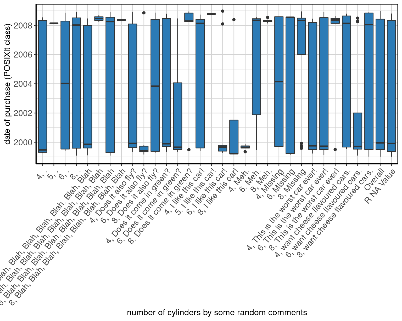
Generate a knitr friendly summary table
make_kable_output(dpltByCylByCommentsSummaryExample)| number of cylinders by some random comments | Label | N | P NA | Mean | S Dev | Med | MAD | 25th P | 75th P | IQR | Min | Max |
|---|---|---|---|---|---|---|---|---|---|---|---|---|
| 4, . | date of purchase (POSIXlt class) | 5 | 0.00 | 2002-12-26 13:38:31 | 260.08 weeks | 1999-06-24 09:05:00 | 17.72 weeks | 1999-04-01 16:49:00 | 2008-05-04 13:32:00 | 474.409028 weeks | 1999-04-01 16:49:00 | 2008-07-19 05:48:36 |
| 6, . | date of purchase (POSIXlt class) | 9 | 11.11 | 2003-12-31 07:58:18 | 247.12 weeks | 2004-01-11 07:48:34 | 340.15 weeks | 1999-06-21 14:04:00 | 2008-05-07 11:07:04 | 463.268161 weeks | 1999-06-01 04:12:00 | 2008-11-12 17:56:39 |
| 8, . | date of purchase (POSIXlt class) | 11 | 0.00 | 2004-05-29 01:24:54 | 245.48 weeks | 2008-01-08 08:48:50 | 69.28 weeks | 1999-06-17 19:51:00 | 2008-06-16 10:15:19 | 469.514317 weeks | 1999-01-31 21:39:00 | 2008-11-30 10:47:06 |
| 4, Blah, Blah, Blah, Blah, Blah, Blah, Blah, Blah | date of purchase (POSIXlt class) | 9 | 0.00 | 2002-06-23 09:51:45 | 223.34 weeks | 1999-11-10 03:37:00 | 28.85 weeks | 1999-06-26 22:47:00 | 2008-01-01 21:17:41 | 444.419711 weeks | 1999-02-06 23:51:00 | 2008-06-22 01:19:06 |
| 6, Blah, Blah, Blah, Blah, Blah, Blah, Blah, Blah | date of purchase (POSIXlt class) | 8 | 12.50 | 2004-07-24 20:46:13 | 261.15 weeks | 2008-04-06 04:33:44 | 50.36 weeks | 1999-03-18 09:04:00 | 2008-09-11 11:16:05 | 495.013103 weeks | 1999-02-02 05:57:00 | 2008-11-29 23:22:31 |
| 8, Blah, Blah, Blah, Blah, Blah, Blah, Blah, Blah | date of purchase (POSIXlt class) | 4 | 50.00 | 2008-05-14 05:42:44 | 2.05 weeks | 2008-05-14 05:42:44 | 2.15 weeks | 2008-05-04 02:11:56 | NA | NA weeks | 2008-05-04 02:11:56 | 2008-05-24 09:13:33 |
| 4, Does it also fly? | date of purchase (POSIXlt class) | 5 | 0.00 | 2003-03-07 13:02:00 | 254.76 weeks | 1999-12-03 14:02:00 | 46.46 weeks | 1999-04-28 06:00:00 | 2008-02-04 15:09:51 | 457.768834 weeks | 1999-04-28 06:00:00 | 2008-12-06 16:25:11 |
| 6, Does it also fly? | date of purchase (POSIXlt class) | 7 | 14.29 | 2000-12-31 00:40:43 | 201.17 weeks | 1999-05-30 16:24:30 | 12.40 weeks | 1999-05-05 05:29:00 | 1999-10-26 17:15:00 | 24.927183 weeks | 1999-02-28 00:08:00 | 2008-11-08 20:23:21 |
| 8, Does it also fly? | date of purchase (POSIXlt class) | 4 | 0.00 | 2003-12-13 22:25:46 | 278.25 weeks | 2003-11-02 13:02:39 | 348.06 weeks | 1999-04-03 04:24:00 | 2008-04-01 21:16:18 | 469.528998 weeks | 1999-04-03 04:24:00 | 2008-11-15 11:13:47 |
| 4, Does it come in green? | date of purchase (POSIXlt class) | 15 | 6.67 | 2003-06-16 06:56:21 | 236.42 weeks | 1999-11-24 15:28:30 | 39.39 weeks | 1999-09-02 05:35:00 | 2008-07-23 15:02:51 | 463.913477 weeks | 1999-05-08 11:54:00 | 2008-10-21 20:32:53 |
| 6, Does it come in green? | date of purchase (POSIXlt class) | 3 | 0.00 | 2002-06-30 08:12:42 | 270.33 weeks | 1999-08-29 03:43:00 | 23.66 weeks | 1999-05-09 11:09:00 | 1999-08-29 03:43:00 | 15.955754 weeks | 1999-05-09 11:09:00 | 2008-06-22 09:46:07 |
| 8, Does it come in green? | date of purchase (POSIXlt class) | 5 | 0.00 | 2006-10-07 03:49:16 | 212.99 weeks | 2008-04-16 09:43:47 | 42.60 weeks | 1999-06-27 01:00:00 | 2008-11-03 12:36:31 | 488.211956 weeks | 1999-06-27 01:00:00 | 2008-12-13 19:57:34 |
| 4, I like this car! | date of purchase (POSIXlt class) | 10 | 0.00 | 2004-11-13 07:26:51 | 239.01 weeks | 2008-02-20 02:59:31 | 43.53 weeks | 1999-07-19 01:45:00 | 2008-06-05 23:16:30 | 463.556696 weeks | 1999-05-25 08:23:00 | 2008-09-27 22:41:44 |
| 6, I like this car! | date of purchase (POSIXlt class) | 9 | 0.00 | 2001-07-09 07:24:32 | 208.13 weeks | 1999-09-01 02:08:00 | 21.11 weeks | 1999-05-20 04:21:00 | 1999-10-17 19:26:00 | 21.518353 weeks | 1999-04-06 04:38:00 | 2008-12-23 01:06:02 |
| 8, I like this car! | date of purchase (POSIXlt class) | 4 | 0.00 | 2001-07-01 15:33:59 | 239.79 weeks | 1999-03-21 09:08:00 | 2.24 weeks | 1999-03-03 10:20:00 | 1999-03-24 14:33:00 | 3.025099 weeks | 1999-03-03 10:20:00 | 2008-05-23 09:39:59 |
| 4, Meh. | date of purchase (POSIXlt class) | 6 | 0.00 | 1999-08-25 12:01:40 | 9.25 weeks | 1999-08-28 23:33:00 | 6.94 weeks | 1999-08-04 16:17:00 | 1999-09-09 16:07:00 | 5.141865 weeks | 1999-05-07 20:04:00 | 1999-11-12 08:41:00 |
| 6, Meh. | date of purchase (POSIXlt class) | 6 | 0.00 | 2005-06-27 05:16:57 | 237.83 weeks | 2008-05-07 15:52:30 | 12.18 weeks | 1999-10-01 21:39:00 | 2008-06-02 21:26:13 | 452.427303 weeks | 1999-06-17 18:37:00 | 2008-07-19 02:28:08 |
| 8, Meh. | date of purchase (POSIXlt class) | 6 | 16.67 | 2008-04-25 09:42:01 | 7.88 weeks | 2008-04-22 03:39:45 | 4.67 weeks | 2008-03-31 02:48:18 | 2008-05-06 10:35:30 | 5.189206 weeks | 2008-02-19 04:00:08 | 2008-07-18 03:26:27 |
| 4, Missing | date of purchase (POSIXlt class) | 6 | 33.33 | 2004-02-24 10:35:52 | 267.91 weeks | 2004-02-24 04:39:56 | 343.94 weeks | 1999-09-16 12:56:00 | 2008-08-08 07:13:36 | 464.108889 weeks | 1999-09-12 01:50:00 | 2008-08-08 07:13:36 |
| 6, Missing | date of purchase (POSIXlt class) | 5 | 0.00 | 2004-10-25 01:13:27 | 267.95 weeks | 2008-07-21 13:26:31 | 2.15 weeks | 1999-02-23 01:03:00 | 2008-07-24 03:53:54 | 491.302669 weeks | 1999-02-23 01:03:00 | 2008-07-31 16:39:54 |
| 8, Missing | date of purchase (POSIXlt class) | 14 | 14.29 | 2006-04-18 06:42:10 | 206.29 weeks | 2008-05-04 22:11:45 | 28.88 weeks | 2008-01-15 10:13:33 | 2008-10-14 02:45:41 | 38.955569 weeks | 1999-08-02 23:23:00 | 2008-12-15 06:26:36 |
| 4, This is the worst car ever! | date of purchase (POSIXlt class) | 7 | 0.00 | 2003-04-05 22:54:10 | 245.37 weeks | 1999-10-03 19:59:00 | 40.91 weeks | 1999-04-01 16:56:00 | 2008-02-06 14:44:36 | 461.844107 weeks | 1999-03-24 16:04:00 | 2008-06-16 19:57:55 |
| 6, This is the worst car ever! | date of purchase (POSIXlt class) | 10 | 10.00 | 2002-08-17 05:20:29 | 241.20 weeks | 1999-09-23 07:05:00 | 31.28 weeks | 1999-04-28 14:16:00 | 2008-11-24 04:28:26 | 499.655995 weeks | 1999-02-22 04:55:00 | 2008-11-29 02:51:30 |
| 8, This is the worst car ever! | date of purchase (POSIXlt class) | 5 | 0.00 | 2006-08-16 08:39:48 | 207.93 weeks | 2008-05-16 14:45:50 | 18.25 weeks | 1999-07-03 07:38:00 | 2008-06-23 13:12:36 | 468.318909 weeks | 1999-07-03 07:38:00 | 2008-08-16 20:36:23 |
| 4, want cheese flavoured cars. | date of purchase (POSIXlt class) | 11 | 36.36 | 2004-09-23 18:01:28 | 249.43 weeks | 2008-02-20 02:52:27 | 51.90 weeks | 1999-09-24 22:41:00 | NA | NA weeks | 1999-07-17 09:42:00 | 2008-10-22 03:49:26 |
| 6, want cheese flavoured cars. | date of purchase (POSIXlt class) | 13 | 7.69 | 2001-10-13 08:39:46 | 206.72 weeks | 1999-09-17 06:54:30 | 16.31 weeks | 1999-07-02 01:34:00 | 2008-04-01 21:06:18 | 456.687728 weeks | 1999-02-02 06:27:00 | 2008-06-29 23:50:43 |
| 8, want cheese flavoured cars. | date of purchase (POSIXlt class) | 9 | 22.22 | 2004-09-01 03:43:02 | 260.61 weeks | 2008-01-19 02:34:35 | 67.07 weeks | 1999-06-20 13:17:00 | 2008-11-30 18:38:11 | 493.031863 weeks | 1999-01-06 16:15:00 | 2008-11-30 18:38:11 |
| Overall | date of purchase (POSIXlt class) | 234 | 8.55 | 2003-11-15 13:01:05 | 234.30 weeks | 1999-12-16 04:23:30 | 67.67 weeks | 1999-07-17 09:42:00 | 2008-07-23 15:02:51 | 470.603259 weeks | 1999-01-04 04:59:00 | 2008-12-23 01:06:02 |
| R NA Value | date of purchase (POSIXlt class) | 24 | 4.17 | 2003-05-14 05:30:18 | 237.27 weeks | 1999-12-02 03:54:00 | 64.95 weeks | 1999-04-07 11:51:00 | 2008-05-14 10:48:26 | 474.993793 weeks | 1999-01-04 04:59:00 | 2008-10-23 18:14:24 |
Generate knitr friendly output
make_complete_output(dpltByCylByCommentsSummaryExample)| number of cylinders by some random comments | Label | N | P NA | Mean | S Dev | Med | MAD | 25th P | 75th P | IQR | Min | Max |
|---|---|---|---|---|---|---|---|---|---|---|---|---|
| 4, . | date of purchase (POSIXlt class) | 5 | 0.00 | 2002-12-26 13:38:31 | 260.08 weeks | 1999-06-24 09:05:00 | 17.72 weeks | 1999-04-01 16:49:00 | 2008-05-04 13:32:00 | 474.409028 weeks | 1999-04-01 16:49:00 | 2008-07-19 05:48:36 |
| 6, . | date of purchase (POSIXlt class) | 9 | 11.11 | 2003-12-31 07:58:18 | 247.12 weeks | 2004-01-11 07:48:34 | 340.15 weeks | 1999-06-21 14:04:00 | 2008-05-07 11:07:04 | 463.268161 weeks | 1999-06-01 04:12:00 | 2008-11-12 17:56:39 |
| 8, . | date of purchase (POSIXlt class) | 11 | 0.00 | 2004-05-29 01:24:54 | 245.48 weeks | 2008-01-08 08:48:50 | 69.28 weeks | 1999-06-17 19:51:00 | 2008-06-16 10:15:19 | 469.514317 weeks | 1999-01-31 21:39:00 | 2008-11-30 10:47:06 |
| 4, Blah, Blah, Blah, Blah, Blah, Blah, Blah, Blah | date of purchase (POSIXlt class) | 9 | 0.00 | 2002-06-23 09:51:45 | 223.34 weeks | 1999-11-10 03:37:00 | 28.85 weeks | 1999-06-26 22:47:00 | 2008-01-01 21:17:41 | 444.419711 weeks | 1999-02-06 23:51:00 | 2008-06-22 01:19:06 |
| 6, Blah, Blah, Blah, Blah, Blah, Blah, Blah, Blah | date of purchase (POSIXlt class) | 8 | 12.50 | 2004-07-24 20:46:13 | 261.15 weeks | 2008-04-06 04:33:44 | 50.36 weeks | 1999-03-18 09:04:00 | 2008-09-11 11:16:05 | 495.013103 weeks | 1999-02-02 05:57:00 | 2008-11-29 23:22:31 |
| 8, Blah, Blah, Blah, Blah, Blah, Blah, Blah, Blah | date of purchase (POSIXlt class) | 4 | 50.00 | 2008-05-14 05:42:44 | 2.05 weeks | 2008-05-14 05:42:44 | 2.15 weeks | 2008-05-04 02:11:56 | NA | NA weeks | 2008-05-04 02:11:56 | 2008-05-24 09:13:33 |
| 4, Does it also fly? | date of purchase (POSIXlt class) | 5 | 0.00 | 2003-03-07 13:02:00 | 254.76 weeks | 1999-12-03 14:02:00 | 46.46 weeks | 1999-04-28 06:00:00 | 2008-02-04 15:09:51 | 457.768834 weeks | 1999-04-28 06:00:00 | 2008-12-06 16:25:11 |
| 6, Does it also fly? | date of purchase (POSIXlt class) | 7 | 14.29 | 2000-12-31 00:40:43 | 201.17 weeks | 1999-05-30 16:24:30 | 12.40 weeks | 1999-05-05 05:29:00 | 1999-10-26 17:15:00 | 24.927183 weeks | 1999-02-28 00:08:00 | 2008-11-08 20:23:21 |
| 8, Does it also fly? | date of purchase (POSIXlt class) | 4 | 0.00 | 2003-12-13 22:25:46 | 278.25 weeks | 2003-11-02 13:02:39 | 348.06 weeks | 1999-04-03 04:24:00 | 2008-04-01 21:16:18 | 469.528998 weeks | 1999-04-03 04:24:00 | 2008-11-15 11:13:47 |
| 4, Does it come in green? | date of purchase (POSIXlt class) | 15 | 6.67 | 2003-06-16 06:56:21 | 236.42 weeks | 1999-11-24 15:28:30 | 39.39 weeks | 1999-09-02 05:35:00 | 2008-07-23 15:02:51 | 463.913477 weeks | 1999-05-08 11:54:00 | 2008-10-21 20:32:53 |
| 6, Does it come in green? | date of purchase (POSIXlt class) | 3 | 0.00 | 2002-06-30 08:12:42 | 270.33 weeks | 1999-08-29 03:43:00 | 23.66 weeks | 1999-05-09 11:09:00 | 1999-08-29 03:43:00 | 15.955754 weeks | 1999-05-09 11:09:00 | 2008-06-22 09:46:07 |
| 8, Does it come in green? | date of purchase (POSIXlt class) | 5 | 0.00 | 2006-10-07 03:49:16 | 212.99 weeks | 2008-04-16 09:43:47 | 42.60 weeks | 1999-06-27 01:00:00 | 2008-11-03 12:36:31 | 488.211956 weeks | 1999-06-27 01:00:00 | 2008-12-13 19:57:34 |
| 4, I like this car! | date of purchase (POSIXlt class) | 10 | 0.00 | 2004-11-13 07:26:51 | 239.01 weeks | 2008-02-20 02:59:31 | 43.53 weeks | 1999-07-19 01:45:00 | 2008-06-05 23:16:30 | 463.556696 weeks | 1999-05-25 08:23:00 | 2008-09-27 22:41:44 |
| 6, I like this car! | date of purchase (POSIXlt class) | 9 | 0.00 | 2001-07-09 07:24:32 | 208.13 weeks | 1999-09-01 02:08:00 | 21.11 weeks | 1999-05-20 04:21:00 | 1999-10-17 19:26:00 | 21.518353 weeks | 1999-04-06 04:38:00 | 2008-12-23 01:06:02 |
| 8, I like this car! | date of purchase (POSIXlt class) | 4 | 0.00 | 2001-07-01 15:33:59 | 239.79 weeks | 1999-03-21 09:08:00 | 2.24 weeks | 1999-03-03 10:20:00 | 1999-03-24 14:33:00 | 3.025099 weeks | 1999-03-03 10:20:00 | 2008-05-23 09:39:59 |
| 4, Meh. | date of purchase (POSIXlt class) | 6 | 0.00 | 1999-08-25 12:01:40 | 9.25 weeks | 1999-08-28 23:33:00 | 6.94 weeks | 1999-08-04 16:17:00 | 1999-09-09 16:07:00 | 5.141865 weeks | 1999-05-07 20:04:00 | 1999-11-12 08:41:00 |
| 6, Meh. | date of purchase (POSIXlt class) | 6 | 0.00 | 2005-06-27 05:16:57 | 237.83 weeks | 2008-05-07 15:52:30 | 12.18 weeks | 1999-10-01 21:39:00 | 2008-06-02 21:26:13 | 452.427303 weeks | 1999-06-17 18:37:00 | 2008-07-19 02:28:08 |
| 8, Meh. | date of purchase (POSIXlt class) | 6 | 16.67 | 2008-04-25 09:42:01 | 7.88 weeks | 2008-04-22 03:39:45 | 4.67 weeks | 2008-03-31 02:48:18 | 2008-05-06 10:35:30 | 5.189206 weeks | 2008-02-19 04:00:08 | 2008-07-18 03:26:27 |
| 4, Missing | date of purchase (POSIXlt class) | 6 | 33.33 | 2004-02-24 10:35:52 | 267.91 weeks | 2004-02-24 04:39:56 | 343.94 weeks | 1999-09-16 12:56:00 | 2008-08-08 07:13:36 | 464.108889 weeks | 1999-09-12 01:50:00 | 2008-08-08 07:13:36 |
| 6, Missing | date of purchase (POSIXlt class) | 5 | 0.00 | 2004-10-25 01:13:27 | 267.95 weeks | 2008-07-21 13:26:31 | 2.15 weeks | 1999-02-23 01:03:00 | 2008-07-24 03:53:54 | 491.302669 weeks | 1999-02-23 01:03:00 | 2008-07-31 16:39:54 |
| 8, Missing | date of purchase (POSIXlt class) | 14 | 14.29 | 2006-04-18 06:42:10 | 206.29 weeks | 2008-05-04 22:11:45 | 28.88 weeks | 2008-01-15 10:13:33 | 2008-10-14 02:45:41 | 38.955569 weeks | 1999-08-02 23:23:00 | 2008-12-15 06:26:36 |
| 4, This is the worst car ever! | date of purchase (POSIXlt class) | 7 | 0.00 | 2003-04-05 22:54:10 | 245.37 weeks | 1999-10-03 19:59:00 | 40.91 weeks | 1999-04-01 16:56:00 | 2008-02-06 14:44:36 | 461.844107 weeks | 1999-03-24 16:04:00 | 2008-06-16 19:57:55 |
| 6, This is the worst car ever! | date of purchase (POSIXlt class) | 10 | 10.00 | 2002-08-17 05:20:29 | 241.20 weeks | 1999-09-23 07:05:00 | 31.28 weeks | 1999-04-28 14:16:00 | 2008-11-24 04:28:26 | 499.655995 weeks | 1999-02-22 04:55:00 | 2008-11-29 02:51:30 |
| 8, This is the worst car ever! | date of purchase (POSIXlt class) | 5 | 0.00 | 2006-08-16 08:39:48 | 207.93 weeks | 2008-05-16 14:45:50 | 18.25 weeks | 1999-07-03 07:38:00 | 2008-06-23 13:12:36 | 468.318909 weeks | 1999-07-03 07:38:00 | 2008-08-16 20:36:23 |
| 4, want cheese flavoured cars. | date of purchase (POSIXlt class) | 11 | 36.36 | 2004-09-23 18:01:28 | 249.43 weeks | 2008-02-20 02:52:27 | 51.90 weeks | 1999-09-24 22:41:00 | NA | NA weeks | 1999-07-17 09:42:00 | 2008-10-22 03:49:26 |
| 6, want cheese flavoured cars. | date of purchase (POSIXlt class) | 13 | 7.69 | 2001-10-13 08:39:46 | 206.72 weeks | 1999-09-17 06:54:30 | 16.31 weeks | 1999-07-02 01:34:00 | 2008-04-01 21:06:18 | 456.687728 weeks | 1999-02-02 06:27:00 | 2008-06-29 23:50:43 |
| 8, want cheese flavoured cars. | date of purchase (POSIXlt class) | 9 | 22.22 | 2004-09-01 03:43:02 | 260.61 weeks | 2008-01-19 02:34:35 | 67.07 weeks | 1999-06-20 13:17:00 | 2008-11-30 18:38:11 | 493.031863 weeks | 1999-01-06 16:15:00 | 2008-11-30 18:38:11 |
| Overall | date of purchase (POSIXlt class) | 234 | 8.55 | 2003-11-15 13:01:05 | 234.30 weeks | 1999-12-16 04:23:30 | 67.67 weeks | 1999-07-17 09:42:00 | 2008-07-23 15:02:51 | 470.603259 weeks | 1999-01-04 04:59:00 | 2008-12-23 01:06:02 |
| R NA Value | date of purchase (POSIXlt class) | 24 | 4.17 | 2003-05-14 05:30:18 | 237.27 weeks | 1999-12-02 03:54:00 | 64.95 weeks | 1999-04-07 11:51:00 | 2008-05-14 10:48:26 | 474.993793 weeks | 1999-01-04 04:59:00 | 2008-10-23 18:14:24 |

Figure 12: Stacked barplot of date of purchase (Date class) by number of cylinders by some random comments.
POSIXct Date
For a date variable x, we need to specify x, the data, and difftime_units.
dpctSummaryExample <- data_summary(x = "dpct", data = mpg, difftime_units = "weeks")Show method to output table and plot
show(dpctSummaryExample)## Label N P NA Mean S Dev
## 1 date of purchase (POSIXct class) 214 8.55 2003-11-21 01:59:50 234.68 weeks
## Med MAD 25th P 75th P
## 1 1999-12-20 21:58:00 71.08 weeks 1999-07-12 05:29:00 2008-08-08 03:44:28
## IQR Min Max
## 1 473.5611 weeks 1999-01-14 10:39:00 2008-12-23 02:41:31
Output the summary table
data_summary_table(dpctSummaryExample)## Label N P NA Mean S Dev
## 1 date of purchase (POSIXct class) 214 8.55 2003-11-21 01:59:50 234.68 weeks
## Med MAD 25th P 75th P
## 1 1999-12-20 21:58:00 71.08 weeks 1999-07-12 05:29:00 2008-08-08 03:44:28
## IQR Min Max
## 1 473.5611 weeks 1999-01-14 10:39:00 2008-12-23 02:41:31Output the plot
data_summary_plot(dpctSummaryExample)
Generate knitr friendly summary table
make_kable_output(dpctSummaryExample)| Label | N | P NA | Mean | S Dev | Med | MAD | 25th P | 75th P | IQR | Min | Max | |
|---|---|---|---|---|---|---|---|---|---|---|---|---|
| date of purchase (POSIXct class) | 214 | 8.55 | 2003-11-21 01:59:50 | 234.68 weeks | 1999-12-20 21:58:00 | 71.08 weeks | 1999-07-12 05:29:00 | 2008-08-08 03:44:28 | 473.5611 weeks | 1999-01-14 10:39:00 | 2008-12-23 02:41:31 |
Generate knitr friendly output
make_complete_output(dpctSummaryExample)| Label | N | P NA | Mean | S Dev | Med | MAD | 25th P | 75th P | IQR | Min | Max | |
|---|---|---|---|---|---|---|---|---|---|---|---|---|
| date of purchase (POSIXct class) | 214 | 8.55 | 2003-11-21 01:59:50 | 234.68 weeks | 1999-12-20 21:58:00 | 71.08 weeks | 1999-07-12 05:29:00 | 2008-08-08 03:44:28 | 473.5611 weeks | 1999-01-14 10:39:00 | 2008-12-23 02:41:31 |
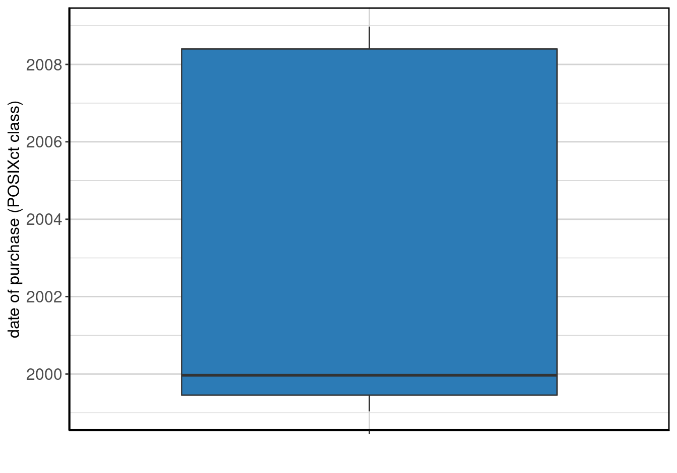
Figure 13: Stacked barplot of date of purchase (Date class).
POSIXct Date By
For a date variable with by, we need to specify x, a by variable, the data, and difftime_units.
dpctByCylSummaryExample <- data_summary(x = "dpct", by = "cyl", data = mpg, difftime_units = "weeks")Show method to output table and plot
show(dpctByCylSummaryExample)## number of cylinders Label N P NA
## 1 4 date of purchase (POSIXct class) 75 7.41
## 2 5 date of purchase (POSIXct class) 3 25.00
## 3 6 date of purchase (POSIXct class) 72 8.86
## 4 8 date of purchase (POSIXct class) 64 8.57
## 5 Overall date of purchase (POSIXct class) 214 8.55
## Mean S Dev Med MAD
## 1 2003-07-18 00:05:46 234.79 weeks 1999-11-04 12:33:00 59.78 weeks
## 2 2008-05-03 15:56:21 22.58 weeks 2008-02-11 11:23:10 3.77 weeks
## 3 2003-02-19 22:01:34 232.07 weeks 1999-11-01 13:42:00 49.24 weeks
## 4 2004-12-05 01:39:52 230.29 weeks 2008-02-22 08:13:23 42.02 weeks
## 5 2003-11-21 01:59:50 234.68 weeks 1999-12-20 21:58:00 71.08 weeks
## 25th P 75th P IQR Min
## 1 1999-06-29 05:05:00 2008-06-13 11:42:47 467.4680 weeks 1999-01-19 10:45:00
## 2 2008-01-24 15:45:51 2008-11-01 20:40:02 40.3149 weeks 2008-01-24 15:45:51
## 3 1999-06-15 01:46:00 2008-07-22 20:44:19 475.1129 weeks 1999-01-19 05:05:00
## 4 1999-09-07 07:18:00 2008-07-30 22:21:17 464.2325 weeks 1999-01-14 10:39:00
## 5 1999-07-12 05:29:00 2008-08-08 03:44:28 473.5611 weeks 1999-01-14 10:39:00
## Max
## 1 2008-12-10 14:15:29
## 2 2008-11-01 20:40:02
## 3 2008-12-19 04:14:10
## 4 2008-12-23 02:41:31
## 5 2008-12-23 02:41:31
Output the summary table
data_summary_table(dpctByCylSummaryExample)## number of cylinders Label N P NA
## 1 4 date of purchase (POSIXct class) 75 7.41
## 2 5 date of purchase (POSIXct class) 3 25.00
## 3 6 date of purchase (POSIXct class) 72 8.86
## 4 8 date of purchase (POSIXct class) 64 8.57
## 5 Overall date of purchase (POSIXct class) 214 8.55
## Mean S Dev Med MAD
## 1 2003-07-18 00:05:46 234.79 weeks 1999-11-04 12:33:00 59.78 weeks
## 2 2008-05-03 15:56:21 22.58 weeks 2008-02-11 11:23:10 3.77 weeks
## 3 2003-02-19 22:01:34 232.07 weeks 1999-11-01 13:42:00 49.24 weeks
## 4 2004-12-05 01:39:52 230.29 weeks 2008-02-22 08:13:23 42.02 weeks
## 5 2003-11-21 01:59:50 234.68 weeks 1999-12-20 21:58:00 71.08 weeks
## 25th P 75th P IQR Min
## 1 1999-06-29 05:05:00 2008-06-13 11:42:47 467.4680 weeks 1999-01-19 10:45:00
## 2 2008-01-24 15:45:51 2008-11-01 20:40:02 40.3149 weeks 2008-01-24 15:45:51
## 3 1999-06-15 01:46:00 2008-07-22 20:44:19 475.1129 weeks 1999-01-19 05:05:00
## 4 1999-09-07 07:18:00 2008-07-30 22:21:17 464.2325 weeks 1999-01-14 10:39:00
## 5 1999-07-12 05:29:00 2008-08-08 03:44:28 473.5611 weeks 1999-01-14 10:39:00
## Max
## 1 2008-12-10 14:15:29
## 2 2008-11-01 20:40:02
## 3 2008-12-19 04:14:10
## 4 2008-12-23 02:41:31
## 5 2008-12-23 02:41:31Output the plot
data_summary_plot(dpctByCylSummaryExample)
Generate a knitr friendly summary table
make_kable_output(dpctByCylSummaryExample)| number of cylinders | Label | N | P NA | Mean | S Dev | Med | MAD | 25th P | 75th P | IQR | Min | Max |
|---|---|---|---|---|---|---|---|---|---|---|---|---|
| 4 | date of purchase (POSIXct class) | 75 | 7.41 | 2003-07-18 00:05:46 | 234.79 weeks | 1999-11-04 12:33:00 | 59.78 weeks | 1999-06-29 05:05:00 | 2008-06-13 11:42:47 | 467.4680 weeks | 1999-01-19 10:45:00 | 2008-12-10 14:15:29 |
| 5 | date of purchase (POSIXct class) | 3 | 25.00 | 2008-05-03 15:56:21 | 22.58 weeks | 2008-02-11 11:23:10 | 3.77 weeks | 2008-01-24 15:45:51 | 2008-11-01 20:40:02 | 40.3149 weeks | 2008-01-24 15:45:51 | 2008-11-01 20:40:02 |
| 6 | date of purchase (POSIXct class) | 72 | 8.86 | 2003-02-19 22:01:34 | 232.07 weeks | 1999-11-01 13:42:00 | 49.24 weeks | 1999-06-15 01:46:00 | 2008-07-22 20:44:19 | 475.1129 weeks | 1999-01-19 05:05:00 | 2008-12-19 04:14:10 |
| 8 | date of purchase (POSIXct class) | 64 | 8.57 | 2004-12-05 01:39:52 | 230.29 weeks | 2008-02-22 08:13:23 | 42.02 weeks | 1999-09-07 07:18:00 | 2008-07-30 22:21:17 | 464.2325 weeks | 1999-01-14 10:39:00 | 2008-12-23 02:41:31 |
| Overall | date of purchase (POSIXct class) | 214 | 8.55 | 2003-11-21 01:59:50 | 234.68 weeks | 1999-12-20 21:58:00 | 71.08 weeks | 1999-07-12 05:29:00 | 2008-08-08 03:44:28 | 473.5611 weeks | 1999-01-14 10:39:00 | 2008-12-23 02:41:31 |
Generate knitr friendly output
make_complete_output(dpctByCylSummaryExample)| number of cylinders | Label | N | P NA | Mean | S Dev | Med | MAD | 25th P | 75th P | IQR | Min | Max |
|---|---|---|---|---|---|---|---|---|---|---|---|---|
| 4 | date of purchase (POSIXct class) | 75 | 7.41 | 2003-07-18 00:05:46 | 234.79 weeks | 1999-11-04 12:33:00 | 59.78 weeks | 1999-06-29 05:05:00 | 2008-06-13 11:42:47 | 467.4680 weeks | 1999-01-19 10:45:00 | 2008-12-10 14:15:29 |
| 5 | date of purchase (POSIXct class) | 3 | 25.00 | 2008-05-03 15:56:21 | 22.58 weeks | 2008-02-11 11:23:10 | 3.77 weeks | 2008-01-24 15:45:51 | 2008-11-01 20:40:02 | 40.3149 weeks | 2008-01-24 15:45:51 | 2008-11-01 20:40:02 |
| 6 | date of purchase (POSIXct class) | 72 | 8.86 | 2003-02-19 22:01:34 | 232.07 weeks | 1999-11-01 13:42:00 | 49.24 weeks | 1999-06-15 01:46:00 | 2008-07-22 20:44:19 | 475.1129 weeks | 1999-01-19 05:05:00 | 2008-12-19 04:14:10 |
| 8 | date of purchase (POSIXct class) | 64 | 8.57 | 2004-12-05 01:39:52 | 230.29 weeks | 2008-02-22 08:13:23 | 42.02 weeks | 1999-09-07 07:18:00 | 2008-07-30 22:21:17 | 464.2325 weeks | 1999-01-14 10:39:00 | 2008-12-23 02:41:31 |
| Overall | date of purchase (POSIXct class) | 214 | 8.55 | 2003-11-21 01:59:50 | 234.68 weeks | 1999-12-20 21:58:00 | 71.08 weeks | 1999-07-12 05:29:00 | 2008-08-08 03:44:28 | 473.5611 weeks | 1999-01-14 10:39:00 | 2008-12-23 02:41:31 |
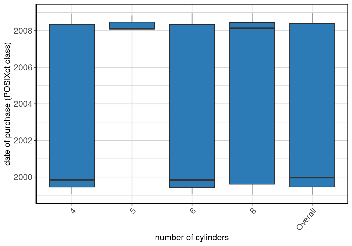
Figure 14: Stacked barplot of date of purchase (Date class) by number of cylinders.
POSIXct Date By By
For a date variable with two or more by variables, we need to specify x, the by variables as a character string, the data, and difftime_units.
dpctByCylByCommentsSummaryExample <- data_summary(x = "dpct", by = c("cyl", "comments"), data = mpg, difftime_units = "weeks")Show method to output table and plot
show(dpctByCylByCommentsSummaryExample)## number of cylinders by some random comments
## 1 4, .
## 2 6, .
## 3 8, .
## 4 4, Blah, Blah, Blah, Blah, Blah, Blah, Blah, Blah
## 5 6, Blah, Blah, Blah, Blah, Blah, Blah, Blah, Blah
## 6 8, Blah, Blah, Blah, Blah, Blah, Blah, Blah, Blah
## 7 4, Does it also fly?
## 8 6, Does it also fly?
## 9 8, Does it also fly?
## 10 4, Does it come in green?
## 11 6, Does it come in green?
## 12 8, Does it come in green?
## 13 4, I like this car!
## 14 6, I like this car!
## 15 8, I like this car!
## 16 4, Meh.
## 17 6, Meh.
## 18 8, Meh.
## 19 4, Missing
## 20 6, Missing
## 21 8, Missing
## 22 4, This is the worst car ever!
## 23 6, This is the worst car ever!
## 24 8, This is the worst car ever!
## 25 4, want cheese flavoured cars.
## 26 6, want cheese flavoured cars.
## 27 8, want cheese flavoured cars.
## 28 Overall
## 29 R NA Value
## Label N P NA Mean S Dev
## 1 date of purchase (POSIXct class) 4 20.00 2003-11-26 01:28:09 264.73 weeks
## 2 date of purchase (POSIXct class) 5 44.44 2002-12-17 07:22:57 270.27 weeks
## 3 date of purchase (POSIXct class) 11 0.00 2004-04-24 18:25:05 249.42 weeks
## 4 date of purchase (POSIXct class) 9 0.00 2002-07-15 11:07:25 241.61 weeks
## 5 date of purchase (POSIXct class) 8 0.00 2005-03-06 05:47:49 242.11 weeks
## 6 date of purchase (POSIXct class) 4 0.00 2004-02-11 02:10:30 276.28 weeks
## 7 date of purchase (POSIXct class) 4 20.00 2001-09-24 20:28:30 248.62 weeks
## 8 date of purchase (POSIXct class) 7 0.00 2002-01-07 00:42:09 233.05 weeks
## 9 date of purchase (POSIXct class) 4 0.00 2003-12-10 08:59:56 274.38 weeks
## 10 date of purchase (POSIXct class) 13 13.33 2004-04-26 17:00:18 242.32 weeks
## 11 date of purchase (POSIXct class) 3 0.00 2002-05-06 16:40:58 282.96 weeks
## 12 date of purchase (POSIXct class) 5 0.00 2006-07-04 18:28:09 202.85 weeks
## 13 date of purchase (POSIXct class) 10 0.00 2004-09-06 10:29:02 236.37 weeks
## 14 date of purchase (POSIXct class) 8 11.11 2001-09-26 14:59:45 221.03 weeks
## 15 date of purchase (POSIXct class) 4 0.00 2001-10-11 20:23:10 217.30 weeks
## 16 date of purchase (POSIXct class) 5 16.67 1999-09-07 15:47:00 10.58 weeks
## 17 date of purchase (POSIXct class) 6 0.00 2005-07-02 00:16:06 239.72 weeks
## 18 date of purchase (POSIXct class) 6 0.00 2008-06-20 06:15:14 15.40 weeks
## 19 date of purchase (POSIXct class) 6 0.00 2005-06-18 03:14:08 242.90 weeks
## 20 date of purchase (POSIXct class) 5 0.00 2004-11-20 04:13:04 261.49 weeks
## 21 date of purchase (POSIXct class) 10 28.57 2005-09-03 04:52:51 232.45 weeks
## 22 date of purchase (POSIXct class) 7 0.00 2003-04-25 21:09:50 251.79 weeks
## 23 date of purchase (POSIXct class) 9 10.00 2002-08-24 04:35:52 231.70 weeks
## 24 date of purchase (POSIXct class) 5 0.00 2006-10-12 09:56:39 199.59 weeks
## 25 date of purchase (POSIXct class) 11 0.00 2003-07-08 16:22:47 243.99 weeks
## 26 date of purchase (POSIXct class) 13 0.00 2002-04-20 12:43:21 220.53 weeks
## 27 date of purchase (POSIXct class) 7 22.22 2004-08-05 02:35:48 242.19 weeks
## 28 date of purchase (POSIXct class) 214 8.55 2003-11-21 01:59:50 234.68 weeks
## 29 date of purchase (POSIXct class) 22 8.33 2003-03-11 06:54:43 237.23 weeks
## Med MAD 25th P 75th P
## 1 2003-11-06 00:13:47 335.21 weeks 1999-05-08 02:24:00 2008-07-25 03:01:02
## 2 1999-03-12 05:37:00 2.16 weeks 1999-03-05 23:19:00 <NA>
## 3 2008-01-13 14:49:44 66.19 weeks 1999-03-07 05:25:00 2008-02-26 03:51:50
## 4 1999-10-27 07:00:00 52.44 weeks 1999-02-21 16:40:00 2008-06-08 18:04:52
## 5 2008-02-29 11:08:42 60.19 weeks 1999-07-29 01:43:00 2008-06-11 19:05:41
## 6 2004-03-28 00:37:14 344.49 weeks 1999-03-12 10:49:00 2008-08-08 03:44:28
## 7 1999-07-02 13:44:30 29.09 weeks 1999-01-25 04:26:00 2008-11-11 01:59:02
## 8 1999-06-15 03:11:00 20.52 weeks 1999-04-08 23:55:00 1999-09-20 00:32:00
## 9 2003-11-28 18:09:45 349.78 weeks 1999-05-04 18:30:00 2008-05-19 16:04:31
## 10 2008-01-30 06:40:31 65.27 weeks 1999-09-11 10:21:00 2008-08-21 11:07:05
## 11 1999-04-10 19:07:00 9.15 weeks 1999-02-26 14:09:00 1999-04-10 19:07:00
## 12 2008-02-18 12:34:57 9.89 weeks 1999-07-23 19:34:00 2008-04-05 05:03:33
## 13 2008-01-15 18:48:46 24.65 weeks 1999-02-03 02:54:00 2008-03-27 13:15:56
## 14 1999-09-15 12:26:30 40.56 weeks 1999-02-28 02:12:00 2008-04-21 14:55:24
## 15 1999-11-08 23:10:00 21.40 weeks 1999-05-23 11:06:00 1999-12-11 11:51:00
## 16 1999-09-08 15:06:00 4.96 weeks 1999-08-16 05:16:00 1999-09-24 04:34:00
## 17 2008-03-20 17:16:55 37.37 weeks 1999-10-04 15:53:00 2008-04-10 14:49:22
## 18 2008-06-07 03:14:04 18.68 weeks 2008-03-11 17:07:43 2008-07-30 22:21:17
## 19 2008-02-16 06:07:01 51.03 weeks 1999-11-09 01:13:00 2008-03-08 08:49:18
## 20 2008-03-11 19:09:42 44.33 weeks 1999-04-04 19:26:00 2008-09-01 07:38:40
## 21 2008-05-08 07:56:16 16.38 weeks 2008-01-19 10:45:49 2008-12-23 02:41:31
## 22 1999-09-09 15:35:00 40.37 weeks 1999-05-18 03:07:00 2008-04-02 21:50:26
## 23 1999-11-23 09:40:00 33.31 weeks 1999-06-19 02:37:00 2008-08-22 22:14:44
## 24 2008-06-06 10:58:47 19.12 weeks 1999-12-12 17:15:00 2008-08-31 04:08:21
## 25 1999-12-19 19:44:00 70.82 weeks 1999-05-29 21:46:00 2008-03-17 00:58:41
## 26 1999-10-22 22:01:00 29.77 weeks 1999-06-04 08:07:00 2008-01-23 02:49:05
## 27 2008-02-12 08:03:24 34.18 weeks 1999-11-17 16:08:00 2008-07-22 16:39:40
## 28 1999-12-20 21:58:00 71.08 weeks 1999-07-12 05:29:00 2008-08-08 03:44:28
## 29 1999-10-23 06:22:30 46.90 weeks 1999-06-05 14:30:00 2008-06-03 01:59:13
## IQR Min Max
## 1 480.860817 weeks 1999-05-08 02:24:00 2008-07-25 03:01:02
## 2 NA weeks 1999-03-02 01:18:00 2008-09-16 09:56:27
## 3 468.276472 weeks 1999-01-21 09:02:00 2008-11-21 02:41:49
## 4 485.008419 weeks 1999-01-20 00:04:00 2008-11-13 01:54:34
## 5 462.960584 weeks 1999-04-21 09:44:00 2008-12-19 04:14:10
## 6 490.957884 weeks 1999-03-12 10:49:00 2008-10-11 20:38:33
## 7 511.128277 weeks 1999-01-25 04:26:00 2008-11-11 01:59:02
## 8 23.432242 weeks 1999-02-22 21:00:00 2008-09-25 23:11:30
## 9 471.842710 weeks 1999-05-04 18:30:00 2008-08-09 05:10:15
## 10 466.718857 weeks 1999-02-13 09:45:00 2008-12-03 10:17:51
## 11 6.172421 weeks 1999-02-26 14:09:00 2008-08-09 16:46:55
## 12 454.056503 weeks 1999-07-23 19:34:00 2008-06-29 09:41:03
## 13 477.204557 weeks 1999-01-26 06:24:00 2008-06-13 11:42:47
## 14 477.218591 weeks 1999-01-19 05:05:00 2008-11-05 13:24:43
## 15 28.861607 weeks 1999-05-23 11:06:00 2008-01-07 00:06:43
## 16 5.567262 weeks 1999-05-30 05:47:00 1999-12-22 00:12:00
## 17 444.422259 weeks 1999-05-28 15:38:00 2008-12-15 14:11:55
## 18 20.173965 weeks 2008-03-05 18:36:33 2008-11-24 17:31:18
## 19 434.616696 weeks 1999-02-03 20:54:00 2008-12-10 14:15:29
## 20 491.072685 weeks 1999-04-04 19:26:00 2008-10-07 02:05:02
## 21 48.380526 weeks 1999-01-14 10:39:00 2008-12-23 02:41:31
## 22 463.254309 weeks 1999-03-03 01:37:00 2008-10-24 23:08:02
## 23 478.973981 weeks 1999-04-03 22:19:00 2008-09-22 00:07:21
## 24 454.921959 weeks 1999-12-12 17:15:00 2008-09-04 17:09:48
## 25 459.161973 weeks 1999-01-19 10:45:00 2008-09-23 14:04:14
## 26 450.682746 weeks 1999-04-04 00:33:00 2008-10-30 14:10:27
## 27 452.860284 weeks 1999-02-27 18:31:00 2008-07-22 16:39:40
## 28 473.561058 weeks 1999-01-14 10:39:00 2008-12-23 02:41:31
## 29 469.354089 weeks 1999-02-12 16:08:00 2008-12-04 06:19:25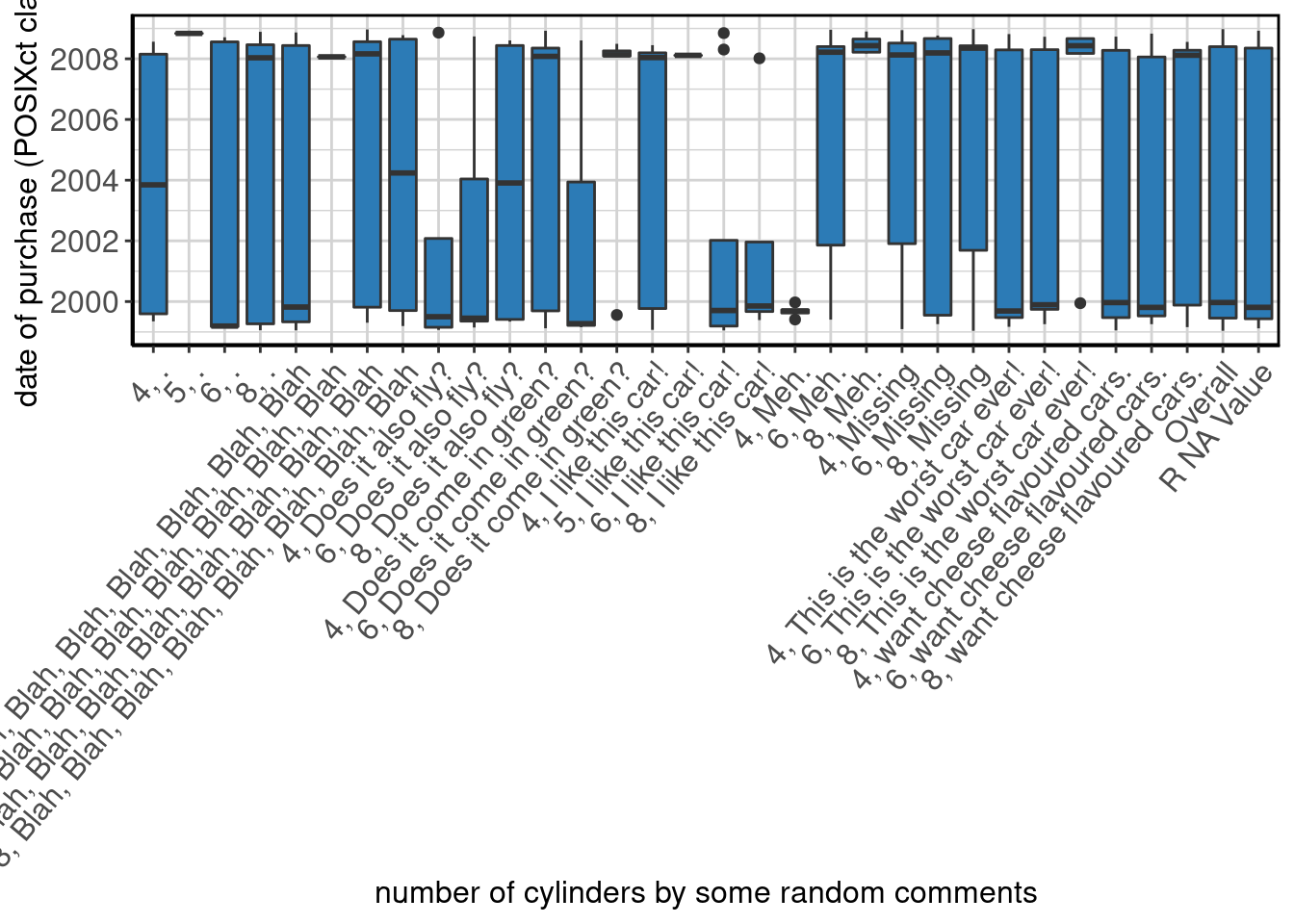
Output the summary table
data_summary_table(dpctByCylByCommentsSummaryExample)## number of cylinders by some random comments
## 1 4, .
## 2 6, .
## 3 8, .
## 4 4, Blah, Blah, Blah, Blah, Blah, Blah, Blah, Blah
## 5 6, Blah, Blah, Blah, Blah, Blah, Blah, Blah, Blah
## 6 8, Blah, Blah, Blah, Blah, Blah, Blah, Blah, Blah
## 7 4, Does it also fly?
## 8 6, Does it also fly?
## 9 8, Does it also fly?
## 10 4, Does it come in green?
## 11 6, Does it come in green?
## 12 8, Does it come in green?
## 13 4, I like this car!
## 14 6, I like this car!
## 15 8, I like this car!
## 16 4, Meh.
## 17 6, Meh.
## 18 8, Meh.
## 19 4, Missing
## 20 6, Missing
## 21 8, Missing
## 22 4, This is the worst car ever!
## 23 6, This is the worst car ever!
## 24 8, This is the worst car ever!
## 25 4, want cheese flavoured cars.
## 26 6, want cheese flavoured cars.
## 27 8, want cheese flavoured cars.
## 28 Overall
## 29 R NA Value
## Label N P NA Mean S Dev
## 1 date of purchase (POSIXct class) 4 20.00 2003-11-26 01:28:09 264.73 weeks
## 2 date of purchase (POSIXct class) 5 44.44 2002-12-17 07:22:57 270.27 weeks
## 3 date of purchase (POSIXct class) 11 0.00 2004-04-24 18:25:05 249.42 weeks
## 4 date of purchase (POSIXct class) 9 0.00 2002-07-15 11:07:25 241.61 weeks
## 5 date of purchase (POSIXct class) 8 0.00 2005-03-06 05:47:49 242.11 weeks
## 6 date of purchase (POSIXct class) 4 0.00 2004-02-11 02:10:30 276.28 weeks
## 7 date of purchase (POSIXct class) 4 20.00 2001-09-24 20:28:30 248.62 weeks
## 8 date of purchase (POSIXct class) 7 0.00 2002-01-07 00:42:09 233.05 weeks
## 9 date of purchase (POSIXct class) 4 0.00 2003-12-10 08:59:56 274.38 weeks
## 10 date of purchase (POSIXct class) 13 13.33 2004-04-26 17:00:18 242.32 weeks
## 11 date of purchase (POSIXct class) 3 0.00 2002-05-06 16:40:58 282.96 weeks
## 12 date of purchase (POSIXct class) 5 0.00 2006-07-04 18:28:09 202.85 weeks
## 13 date of purchase (POSIXct class) 10 0.00 2004-09-06 10:29:02 236.37 weeks
## 14 date of purchase (POSIXct class) 8 11.11 2001-09-26 14:59:45 221.03 weeks
## 15 date of purchase (POSIXct class) 4 0.00 2001-10-11 20:23:10 217.30 weeks
## 16 date of purchase (POSIXct class) 5 16.67 1999-09-07 15:47:00 10.58 weeks
## 17 date of purchase (POSIXct class) 6 0.00 2005-07-02 00:16:06 239.72 weeks
## 18 date of purchase (POSIXct class) 6 0.00 2008-06-20 06:15:14 15.40 weeks
## 19 date of purchase (POSIXct class) 6 0.00 2005-06-18 03:14:08 242.90 weeks
## 20 date of purchase (POSIXct class) 5 0.00 2004-11-20 04:13:04 261.49 weeks
## 21 date of purchase (POSIXct class) 10 28.57 2005-09-03 04:52:51 232.45 weeks
## 22 date of purchase (POSIXct class) 7 0.00 2003-04-25 21:09:50 251.79 weeks
## 23 date of purchase (POSIXct class) 9 10.00 2002-08-24 04:35:52 231.70 weeks
## 24 date of purchase (POSIXct class) 5 0.00 2006-10-12 09:56:39 199.59 weeks
## 25 date of purchase (POSIXct class) 11 0.00 2003-07-08 16:22:47 243.99 weeks
## 26 date of purchase (POSIXct class) 13 0.00 2002-04-20 12:43:21 220.53 weeks
## 27 date of purchase (POSIXct class) 7 22.22 2004-08-05 02:35:48 242.19 weeks
## 28 date of purchase (POSIXct class) 214 8.55 2003-11-21 01:59:50 234.68 weeks
## 29 date of purchase (POSIXct class) 22 8.33 2003-03-11 06:54:43 237.23 weeks
## Med MAD 25th P 75th P
## 1 2003-11-06 00:13:47 335.21 weeks 1999-05-08 02:24:00 2008-07-25 03:01:02
## 2 1999-03-12 05:37:00 2.16 weeks 1999-03-05 23:19:00 <NA>
## 3 2008-01-13 14:49:44 66.19 weeks 1999-03-07 05:25:00 2008-02-26 03:51:50
## 4 1999-10-27 07:00:00 52.44 weeks 1999-02-21 16:40:00 2008-06-08 18:04:52
## 5 2008-02-29 11:08:42 60.19 weeks 1999-07-29 01:43:00 2008-06-11 19:05:41
## 6 2004-03-28 00:37:14 344.49 weeks 1999-03-12 10:49:00 2008-08-08 03:44:28
## 7 1999-07-02 13:44:30 29.09 weeks 1999-01-25 04:26:00 2008-11-11 01:59:02
## 8 1999-06-15 03:11:00 20.52 weeks 1999-04-08 23:55:00 1999-09-20 00:32:00
## 9 2003-11-28 18:09:45 349.78 weeks 1999-05-04 18:30:00 2008-05-19 16:04:31
## 10 2008-01-30 06:40:31 65.27 weeks 1999-09-11 10:21:00 2008-08-21 11:07:05
## 11 1999-04-10 19:07:00 9.15 weeks 1999-02-26 14:09:00 1999-04-10 19:07:00
## 12 2008-02-18 12:34:57 9.89 weeks 1999-07-23 19:34:00 2008-04-05 05:03:33
## 13 2008-01-15 18:48:46 24.65 weeks 1999-02-03 02:54:00 2008-03-27 13:15:56
## 14 1999-09-15 12:26:30 40.56 weeks 1999-02-28 02:12:00 2008-04-21 14:55:24
## 15 1999-11-08 23:10:00 21.40 weeks 1999-05-23 11:06:00 1999-12-11 11:51:00
## 16 1999-09-08 15:06:00 4.96 weeks 1999-08-16 05:16:00 1999-09-24 04:34:00
## 17 2008-03-20 17:16:55 37.37 weeks 1999-10-04 15:53:00 2008-04-10 14:49:22
## 18 2008-06-07 03:14:04 18.68 weeks 2008-03-11 17:07:43 2008-07-30 22:21:17
## 19 2008-02-16 06:07:01 51.03 weeks 1999-11-09 01:13:00 2008-03-08 08:49:18
## 20 2008-03-11 19:09:42 44.33 weeks 1999-04-04 19:26:00 2008-09-01 07:38:40
## 21 2008-05-08 07:56:16 16.38 weeks 2008-01-19 10:45:49 2008-12-23 02:41:31
## 22 1999-09-09 15:35:00 40.37 weeks 1999-05-18 03:07:00 2008-04-02 21:50:26
## 23 1999-11-23 09:40:00 33.31 weeks 1999-06-19 02:37:00 2008-08-22 22:14:44
## 24 2008-06-06 10:58:47 19.12 weeks 1999-12-12 17:15:00 2008-08-31 04:08:21
## 25 1999-12-19 19:44:00 70.82 weeks 1999-05-29 21:46:00 2008-03-17 00:58:41
## 26 1999-10-22 22:01:00 29.77 weeks 1999-06-04 08:07:00 2008-01-23 02:49:05
## 27 2008-02-12 08:03:24 34.18 weeks 1999-11-17 16:08:00 2008-07-22 16:39:40
## 28 1999-12-20 21:58:00 71.08 weeks 1999-07-12 05:29:00 2008-08-08 03:44:28
## 29 1999-10-23 06:22:30 46.90 weeks 1999-06-05 14:30:00 2008-06-03 01:59:13
## IQR Min Max
## 1 480.860817 weeks 1999-05-08 02:24:00 2008-07-25 03:01:02
## 2 NA weeks 1999-03-02 01:18:00 2008-09-16 09:56:27
## 3 468.276472 weeks 1999-01-21 09:02:00 2008-11-21 02:41:49
## 4 485.008419 weeks 1999-01-20 00:04:00 2008-11-13 01:54:34
## 5 462.960584 weeks 1999-04-21 09:44:00 2008-12-19 04:14:10
## 6 490.957884 weeks 1999-03-12 10:49:00 2008-10-11 20:38:33
## 7 511.128277 weeks 1999-01-25 04:26:00 2008-11-11 01:59:02
## 8 23.432242 weeks 1999-02-22 21:00:00 2008-09-25 23:11:30
## 9 471.842710 weeks 1999-05-04 18:30:00 2008-08-09 05:10:15
## 10 466.718857 weeks 1999-02-13 09:45:00 2008-12-03 10:17:51
## 11 6.172421 weeks 1999-02-26 14:09:00 2008-08-09 16:46:55
## 12 454.056503 weeks 1999-07-23 19:34:00 2008-06-29 09:41:03
## 13 477.204557 weeks 1999-01-26 06:24:00 2008-06-13 11:42:47
## 14 477.218591 weeks 1999-01-19 05:05:00 2008-11-05 13:24:43
## 15 28.861607 weeks 1999-05-23 11:06:00 2008-01-07 00:06:43
## 16 5.567262 weeks 1999-05-30 05:47:00 1999-12-22 00:12:00
## 17 444.422259 weeks 1999-05-28 15:38:00 2008-12-15 14:11:55
## 18 20.173965 weeks 2008-03-05 18:36:33 2008-11-24 17:31:18
## 19 434.616696 weeks 1999-02-03 20:54:00 2008-12-10 14:15:29
## 20 491.072685 weeks 1999-04-04 19:26:00 2008-10-07 02:05:02
## 21 48.380526 weeks 1999-01-14 10:39:00 2008-12-23 02:41:31
## 22 463.254309 weeks 1999-03-03 01:37:00 2008-10-24 23:08:02
## 23 478.973981 weeks 1999-04-03 22:19:00 2008-09-22 00:07:21
## 24 454.921959 weeks 1999-12-12 17:15:00 2008-09-04 17:09:48
## 25 459.161973 weeks 1999-01-19 10:45:00 2008-09-23 14:04:14
## 26 450.682746 weeks 1999-04-04 00:33:00 2008-10-30 14:10:27
## 27 452.860284 weeks 1999-02-27 18:31:00 2008-07-22 16:39:40
## 28 473.561058 weeks 1999-01-14 10:39:00 2008-12-23 02:41:31
## 29 469.354089 weeks 1999-02-12 16:08:00 2008-12-04 06:19:25Output the plot
data_summary_plot(dpctByCylByCommentsSummaryExample)
Generate a knitr friendly summary table
make_kable_output(dpctByCylByCommentsSummaryExample)| number of cylinders by some random comments | Label | N | P NA | Mean | S Dev | Med | MAD | 25th P | 75th P | IQR | Min | Max |
|---|---|---|---|---|---|---|---|---|---|---|---|---|
| 4, . | date of purchase (POSIXct class) | 4 | 20.00 | 2003-11-26 01:28:09 | 264.73 weeks | 2003-11-06 00:13:47 | 335.21 weeks | 1999-05-08 02:24:00 | 2008-07-25 03:01:02 | 480.860817 weeks | 1999-05-08 02:24:00 | 2008-07-25 03:01:02 |
| 6, . | date of purchase (POSIXct class) | 5 | 44.44 | 2002-12-17 07:22:57 | 270.27 weeks | 1999-03-12 05:37:00 | 2.16 weeks | 1999-03-05 23:19:00 | NA | NA weeks | 1999-03-02 01:18:00 | 2008-09-16 09:56:27 |
| 8, . | date of purchase (POSIXct class) | 11 | 0.00 | 2004-04-24 18:25:05 | 249.42 weeks | 2008-01-13 14:49:44 | 66.19 weeks | 1999-03-07 05:25:00 | 2008-02-26 03:51:50 | 468.276472 weeks | 1999-01-21 09:02:00 | 2008-11-21 02:41:49 |
| 4, Blah, Blah, Blah, Blah, Blah, Blah, Blah, Blah | date of purchase (POSIXct class) | 9 | 0.00 | 2002-07-15 11:07:25 | 241.61 weeks | 1999-10-27 07:00:00 | 52.44 weeks | 1999-02-21 16:40:00 | 2008-06-08 18:04:52 | 485.008419 weeks | 1999-01-20 00:04:00 | 2008-11-13 01:54:34 |
| 6, Blah, Blah, Blah, Blah, Blah, Blah, Blah, Blah | date of purchase (POSIXct class) | 8 | 0.00 | 2005-03-06 05:47:49 | 242.11 weeks | 2008-02-29 11:08:42 | 60.19 weeks | 1999-07-29 01:43:00 | 2008-06-11 19:05:41 | 462.960584 weeks | 1999-04-21 09:44:00 | 2008-12-19 04:14:10 |
| 8, Blah, Blah, Blah, Blah, Blah, Blah, Blah, Blah | date of purchase (POSIXct class) | 4 | 0.00 | 2004-02-11 02:10:30 | 276.28 weeks | 2004-03-28 00:37:14 | 344.49 weeks | 1999-03-12 10:49:00 | 2008-08-08 03:44:28 | 490.957884 weeks | 1999-03-12 10:49:00 | 2008-10-11 20:38:33 |
| 4, Does it also fly? | date of purchase (POSIXct class) | 4 | 20.00 | 2001-09-24 20:28:30 | 248.62 weeks | 1999-07-02 13:44:30 | 29.09 weeks | 1999-01-25 04:26:00 | 2008-11-11 01:59:02 | 511.128277 weeks | 1999-01-25 04:26:00 | 2008-11-11 01:59:02 |
| 6, Does it also fly? | date of purchase (POSIXct class) | 7 | 0.00 | 2002-01-07 00:42:09 | 233.05 weeks | 1999-06-15 03:11:00 | 20.52 weeks | 1999-04-08 23:55:00 | 1999-09-20 00:32:00 | 23.432242 weeks | 1999-02-22 21:00:00 | 2008-09-25 23:11:30 |
| 8, Does it also fly? | date of purchase (POSIXct class) | 4 | 0.00 | 2003-12-10 08:59:56 | 274.38 weeks | 2003-11-28 18:09:45 | 349.78 weeks | 1999-05-04 18:30:00 | 2008-05-19 16:04:31 | 471.842710 weeks | 1999-05-04 18:30:00 | 2008-08-09 05:10:15 |
| 4, Does it come in green? | date of purchase (POSIXct class) | 13 | 13.33 | 2004-04-26 17:00:18 | 242.32 weeks | 2008-01-30 06:40:31 | 65.27 weeks | 1999-09-11 10:21:00 | 2008-08-21 11:07:05 | 466.718858 weeks | 1999-02-13 09:45:00 | 2008-12-03 10:17:51 |
| 6, Does it come in green? | date of purchase (POSIXct class) | 3 | 0.00 | 2002-05-06 16:40:58 | 282.96 weeks | 1999-04-10 19:07:00 | 9.15 weeks | 1999-02-26 14:09:00 | 1999-04-10 19:07:00 | 6.172421 weeks | 1999-02-26 14:09:00 | 2008-08-09 16:46:55 |
| 8, Does it come in green? | date of purchase (POSIXct class) | 5 | 0.00 | 2006-07-04 18:28:09 | 202.85 weeks | 2008-02-18 12:34:57 | 9.89 weeks | 1999-07-23 19:34:00 | 2008-04-05 05:03:33 | 454.056503 weeks | 1999-07-23 19:34:00 | 2008-06-29 09:41:03 |
| 4, I like this car! | date of purchase (POSIXct class) | 10 | 0.00 | 2004-09-06 10:29:02 | 236.37 weeks | 2008-01-15 18:48:46 | 24.65 weeks | 1999-02-03 02:54:00 | 2008-03-27 13:15:56 | 477.204557 weeks | 1999-01-26 06:24:00 | 2008-06-13 11:42:47 |
| 6, I like this car! | date of purchase (POSIXct class) | 8 | 11.11 | 2001-09-26 14:59:45 | 221.03 weeks | 1999-09-15 12:26:30 | 40.56 weeks | 1999-02-28 02:12:00 | 2008-04-21 14:55:24 | 477.218591 weeks | 1999-01-19 05:05:00 | 2008-11-05 13:24:43 |
| 8, I like this car! | date of purchase (POSIXct class) | 4 | 0.00 | 2001-10-11 20:23:10 | 217.30 weeks | 1999-11-08 23:10:00 | 21.40 weeks | 1999-05-23 11:06:00 | 1999-12-11 11:51:00 | 28.861607 weeks | 1999-05-23 11:06:00 | 2008-01-07 00:06:43 |
| 4, Meh. | date of purchase (POSIXct class) | 5 | 16.67 | 1999-09-07 15:47:00 | 10.58 weeks | 1999-09-08 15:06:00 | 4.96 weeks | 1999-08-16 05:16:00 | 1999-09-24 04:34:00 | 5.567262 weeks | 1999-05-30 05:47:00 | 1999-12-22 00:12:00 |
| 6, Meh. | date of purchase (POSIXct class) | 6 | 0.00 | 2005-07-02 00:16:06 | 239.72 weeks | 2008-03-20 17:16:55 | 37.37 weeks | 1999-10-04 15:53:00 | 2008-04-10 14:49:22 | 444.422259 weeks | 1999-05-28 15:38:00 | 2008-12-15 14:11:55 |
| 8, Meh. | date of purchase (POSIXct class) | 6 | 0.00 | 2008-06-20 06:15:14 | 15.40 weeks | 2008-06-07 03:14:04 | 18.68 weeks | 2008-03-11 17:07:43 | 2008-07-30 22:21:17 | 20.173965 weeks | 2008-03-05 18:36:33 | 2008-11-24 17:31:18 |
| 4, Missing | date of purchase (POSIXct class) | 6 | 0.00 | 2005-06-18 03:14:08 | 242.90 weeks | 2008-02-16 06:07:01 | 51.03 weeks | 1999-11-09 01:13:00 | 2008-03-08 08:49:18 | 434.616696 weeks | 1999-02-03 20:54:00 | 2008-12-10 14:15:29 |
| 6, Missing | date of purchase (POSIXct class) | 5 | 0.00 | 2004-11-20 04:13:04 | 261.49 weeks | 2008-03-11 19:09:42 | 44.33 weeks | 1999-04-04 19:26:00 | 2008-09-01 07:38:40 | 491.072685 weeks | 1999-04-04 19:26:00 | 2008-10-07 02:05:02 |
| 8, Missing | date of purchase (POSIXct class) | 10 | 28.57 | 2005-09-03 04:52:51 | 232.45 weeks | 2008-05-08 07:56:16 | 16.38 weeks | 2008-01-19 10:45:49 | 2008-12-23 02:41:31 | 48.380526 weeks | 1999-01-14 10:39:00 | 2008-12-23 02:41:31 |
| 4, This is the worst car ever! | date of purchase (POSIXct class) | 7 | 0.00 | 2003-04-25 21:09:50 | 251.79 weeks | 1999-09-09 15:35:00 | 40.37 weeks | 1999-05-18 03:07:00 | 2008-04-02 21:50:26 | 463.254309 weeks | 1999-03-03 01:37:00 | 2008-10-24 23:08:02 |
| 6, This is the worst car ever! | date of purchase (POSIXct class) | 9 | 10.00 | 2002-08-24 04:35:52 | 231.70 weeks | 1999-11-23 09:40:00 | 33.31 weeks | 1999-06-19 02:37:00 | 2008-08-22 22:14:44 | 478.973981 weeks | 1999-04-03 22:19:00 | 2008-09-22 00:07:21 |
| 8, This is the worst car ever! | date of purchase (POSIXct class) | 5 | 0.00 | 2006-10-12 09:56:39 | 199.59 weeks | 2008-06-06 10:58:47 | 19.12 weeks | 1999-12-12 17:15:00 | 2008-08-31 04:08:21 | 454.921959 weeks | 1999-12-12 17:15:00 | 2008-09-04 17:09:48 |
| 4, want cheese flavoured cars. | date of purchase (POSIXct class) | 11 | 0.00 | 2003-07-08 16:22:47 | 243.99 weeks | 1999-12-19 19:44:00 | 70.82 weeks | 1999-05-29 21:46:00 | 2008-03-17 00:58:41 | 459.161973 weeks | 1999-01-19 10:45:00 | 2008-09-23 14:04:14 |
| 6, want cheese flavoured cars. | date of purchase (POSIXct class) | 13 | 0.00 | 2002-04-20 12:43:21 | 220.53 weeks | 1999-10-22 22:01:00 | 29.77 weeks | 1999-06-04 08:07:00 | 2008-01-23 02:49:05 | 450.682746 weeks | 1999-04-04 00:33:00 | 2008-10-30 14:10:27 |
| 8, want cheese flavoured cars. | date of purchase (POSIXct class) | 7 | 22.22 | 2004-08-05 02:35:48 | 242.19 weeks | 2008-02-12 08:03:24 | 34.18 weeks | 1999-11-17 16:08:00 | 2008-07-22 16:39:40 | 452.860284 weeks | 1999-02-27 18:31:00 | 2008-07-22 16:39:40 |
| Overall | date of purchase (POSIXct class) | 214 | 8.55 | 2003-11-21 01:59:50 | 234.68 weeks | 1999-12-20 21:58:00 | 71.08 weeks | 1999-07-12 05:29:00 | 2008-08-08 03:44:28 | 473.561058 weeks | 1999-01-14 10:39:00 | 2008-12-23 02:41:31 |
| R NA Value | date of purchase (POSIXct class) | 22 | 8.33 | 2003-03-11 06:54:43 | 237.23 weeks | 1999-10-23 06:22:30 | 46.90 weeks | 1999-06-05 14:30:00 | 2008-06-03 01:59:13 | 469.354089 weeks | 1999-02-12 16:08:00 | 2008-12-04 06:19:25 |
Generate knitr friendly output
make_complete_output(dpctByCylByCommentsSummaryExample)| number of cylinders by some random comments | Label | N | P NA | Mean | S Dev | Med | MAD | 25th P | 75th P | IQR | Min | Max |
|---|---|---|---|---|---|---|---|---|---|---|---|---|
| 4, . | date of purchase (POSIXct class) | 4 | 20.00 | 2003-11-26 01:28:09 | 264.73 weeks | 2003-11-06 00:13:47 | 335.21 weeks | 1999-05-08 02:24:00 | 2008-07-25 03:01:02 | 480.860817 weeks | 1999-05-08 02:24:00 | 2008-07-25 03:01:02 |
| 6, . | date of purchase (POSIXct class) | 5 | 44.44 | 2002-12-17 07:22:57 | 270.27 weeks | 1999-03-12 05:37:00 | 2.16 weeks | 1999-03-05 23:19:00 | NA | NA weeks | 1999-03-02 01:18:00 | 2008-09-16 09:56:27 |
| 8, . | date of purchase (POSIXct class) | 11 | 0.00 | 2004-04-24 18:25:05 | 249.42 weeks | 2008-01-13 14:49:44 | 66.19 weeks | 1999-03-07 05:25:00 | 2008-02-26 03:51:50 | 468.276472 weeks | 1999-01-21 09:02:00 | 2008-11-21 02:41:49 |
| 4, Blah, Blah, Blah, Blah, Blah, Blah, Blah, Blah | date of purchase (POSIXct class) | 9 | 0.00 | 2002-07-15 11:07:25 | 241.61 weeks | 1999-10-27 07:00:00 | 52.44 weeks | 1999-02-21 16:40:00 | 2008-06-08 18:04:52 | 485.008419 weeks | 1999-01-20 00:04:00 | 2008-11-13 01:54:34 |
| 6, Blah, Blah, Blah, Blah, Blah, Blah, Blah, Blah | date of purchase (POSIXct class) | 8 | 0.00 | 2005-03-06 05:47:49 | 242.11 weeks | 2008-02-29 11:08:42 | 60.19 weeks | 1999-07-29 01:43:00 | 2008-06-11 19:05:41 | 462.960584 weeks | 1999-04-21 09:44:00 | 2008-12-19 04:14:10 |
| 8, Blah, Blah, Blah, Blah, Blah, Blah, Blah, Blah | date of purchase (POSIXct class) | 4 | 0.00 | 2004-02-11 02:10:30 | 276.28 weeks | 2004-03-28 00:37:14 | 344.49 weeks | 1999-03-12 10:49:00 | 2008-08-08 03:44:28 | 490.957884 weeks | 1999-03-12 10:49:00 | 2008-10-11 20:38:33 |
| 4, Does it also fly? | date of purchase (POSIXct class) | 4 | 20.00 | 2001-09-24 20:28:30 | 248.62 weeks | 1999-07-02 13:44:30 | 29.09 weeks | 1999-01-25 04:26:00 | 2008-11-11 01:59:02 | 511.128277 weeks | 1999-01-25 04:26:00 | 2008-11-11 01:59:02 |
| 6, Does it also fly? | date of purchase (POSIXct class) | 7 | 0.00 | 2002-01-07 00:42:09 | 233.05 weeks | 1999-06-15 03:11:00 | 20.52 weeks | 1999-04-08 23:55:00 | 1999-09-20 00:32:00 | 23.432242 weeks | 1999-02-22 21:00:00 | 2008-09-25 23:11:30 |
| 8, Does it also fly? | date of purchase (POSIXct class) | 4 | 0.00 | 2003-12-10 08:59:56 | 274.38 weeks | 2003-11-28 18:09:45 | 349.78 weeks | 1999-05-04 18:30:00 | 2008-05-19 16:04:31 | 471.842710 weeks | 1999-05-04 18:30:00 | 2008-08-09 05:10:15 |
| 4, Does it come in green? | date of purchase (POSIXct class) | 13 | 13.33 | 2004-04-26 17:00:18 | 242.32 weeks | 2008-01-30 06:40:31 | 65.27 weeks | 1999-09-11 10:21:00 | 2008-08-21 11:07:05 | 466.718858 weeks | 1999-02-13 09:45:00 | 2008-12-03 10:17:51 |
| 6, Does it come in green? | date of purchase (POSIXct class) | 3 | 0.00 | 2002-05-06 16:40:58 | 282.96 weeks | 1999-04-10 19:07:00 | 9.15 weeks | 1999-02-26 14:09:00 | 1999-04-10 19:07:00 | 6.172421 weeks | 1999-02-26 14:09:00 | 2008-08-09 16:46:55 |
| 8, Does it come in green? | date of purchase (POSIXct class) | 5 | 0.00 | 2006-07-04 18:28:09 | 202.85 weeks | 2008-02-18 12:34:57 | 9.89 weeks | 1999-07-23 19:34:00 | 2008-04-05 05:03:33 | 454.056503 weeks | 1999-07-23 19:34:00 | 2008-06-29 09:41:03 |
| 4, I like this car! | date of purchase (POSIXct class) | 10 | 0.00 | 2004-09-06 10:29:02 | 236.37 weeks | 2008-01-15 18:48:46 | 24.65 weeks | 1999-02-03 02:54:00 | 2008-03-27 13:15:56 | 477.204557 weeks | 1999-01-26 06:24:00 | 2008-06-13 11:42:47 |
| 6, I like this car! | date of purchase (POSIXct class) | 8 | 11.11 | 2001-09-26 14:59:45 | 221.03 weeks | 1999-09-15 12:26:30 | 40.56 weeks | 1999-02-28 02:12:00 | 2008-04-21 14:55:24 | 477.218591 weeks | 1999-01-19 05:05:00 | 2008-11-05 13:24:43 |
| 8, I like this car! | date of purchase (POSIXct class) | 4 | 0.00 | 2001-10-11 20:23:10 | 217.30 weeks | 1999-11-08 23:10:00 | 21.40 weeks | 1999-05-23 11:06:00 | 1999-12-11 11:51:00 | 28.861607 weeks | 1999-05-23 11:06:00 | 2008-01-07 00:06:43 |
| 4, Meh. | date of purchase (POSIXct class) | 5 | 16.67 | 1999-09-07 15:47:00 | 10.58 weeks | 1999-09-08 15:06:00 | 4.96 weeks | 1999-08-16 05:16:00 | 1999-09-24 04:34:00 | 5.567262 weeks | 1999-05-30 05:47:00 | 1999-12-22 00:12:00 |
| 6, Meh. | date of purchase (POSIXct class) | 6 | 0.00 | 2005-07-02 00:16:06 | 239.72 weeks | 2008-03-20 17:16:55 | 37.37 weeks | 1999-10-04 15:53:00 | 2008-04-10 14:49:22 | 444.422259 weeks | 1999-05-28 15:38:00 | 2008-12-15 14:11:55 |
| 8, Meh. | date of purchase (POSIXct class) | 6 | 0.00 | 2008-06-20 06:15:14 | 15.40 weeks | 2008-06-07 03:14:04 | 18.68 weeks | 2008-03-11 17:07:43 | 2008-07-30 22:21:17 | 20.173965 weeks | 2008-03-05 18:36:33 | 2008-11-24 17:31:18 |
| 4, Missing | date of purchase (POSIXct class) | 6 | 0.00 | 2005-06-18 03:14:08 | 242.90 weeks | 2008-02-16 06:07:01 | 51.03 weeks | 1999-11-09 01:13:00 | 2008-03-08 08:49:18 | 434.616696 weeks | 1999-02-03 20:54:00 | 2008-12-10 14:15:29 |
| 6, Missing | date of purchase (POSIXct class) | 5 | 0.00 | 2004-11-20 04:13:04 | 261.49 weeks | 2008-03-11 19:09:42 | 44.33 weeks | 1999-04-04 19:26:00 | 2008-09-01 07:38:40 | 491.072685 weeks | 1999-04-04 19:26:00 | 2008-10-07 02:05:02 |
| 8, Missing | date of purchase (POSIXct class) | 10 | 28.57 | 2005-09-03 04:52:51 | 232.45 weeks | 2008-05-08 07:56:16 | 16.38 weeks | 2008-01-19 10:45:49 | 2008-12-23 02:41:31 | 48.380526 weeks | 1999-01-14 10:39:00 | 2008-12-23 02:41:31 |
| 4, This is the worst car ever! | date of purchase (POSIXct class) | 7 | 0.00 | 2003-04-25 21:09:50 | 251.79 weeks | 1999-09-09 15:35:00 | 40.37 weeks | 1999-05-18 03:07:00 | 2008-04-02 21:50:26 | 463.254309 weeks | 1999-03-03 01:37:00 | 2008-10-24 23:08:02 |
| 6, This is the worst car ever! | date of purchase (POSIXct class) | 9 | 10.00 | 2002-08-24 04:35:52 | 231.70 weeks | 1999-11-23 09:40:00 | 33.31 weeks | 1999-06-19 02:37:00 | 2008-08-22 22:14:44 | 478.973981 weeks | 1999-04-03 22:19:00 | 2008-09-22 00:07:21 |
| 8, This is the worst car ever! | date of purchase (POSIXct class) | 5 | 0.00 | 2006-10-12 09:56:39 | 199.59 weeks | 2008-06-06 10:58:47 | 19.12 weeks | 1999-12-12 17:15:00 | 2008-08-31 04:08:21 | 454.921959 weeks | 1999-12-12 17:15:00 | 2008-09-04 17:09:48 |
| 4, want cheese flavoured cars. | date of purchase (POSIXct class) | 11 | 0.00 | 2003-07-08 16:22:47 | 243.99 weeks | 1999-12-19 19:44:00 | 70.82 weeks | 1999-05-29 21:46:00 | 2008-03-17 00:58:41 | 459.161973 weeks | 1999-01-19 10:45:00 | 2008-09-23 14:04:14 |
| 6, want cheese flavoured cars. | date of purchase (POSIXct class) | 13 | 0.00 | 2002-04-20 12:43:21 | 220.53 weeks | 1999-10-22 22:01:00 | 29.77 weeks | 1999-06-04 08:07:00 | 2008-01-23 02:49:05 | 450.682746 weeks | 1999-04-04 00:33:00 | 2008-10-30 14:10:27 |
| 8, want cheese flavoured cars. | date of purchase (POSIXct class) | 7 | 22.22 | 2004-08-05 02:35:48 | 242.19 weeks | 2008-02-12 08:03:24 | 34.18 weeks | 1999-11-17 16:08:00 | 2008-07-22 16:39:40 | 452.860284 weeks | 1999-02-27 18:31:00 | 2008-07-22 16:39:40 |
| Overall | date of purchase (POSIXct class) | 214 | 8.55 | 2003-11-21 01:59:50 | 234.68 weeks | 1999-12-20 21:58:00 | 71.08 weeks | 1999-07-12 05:29:00 | 2008-08-08 03:44:28 | 473.561058 weeks | 1999-01-14 10:39:00 | 2008-12-23 02:41:31 |
| R NA Value | date of purchase (POSIXct class) | 22 | 8.33 | 2003-03-11 06:54:43 | 237.23 weeks | 1999-10-23 06:22:30 | 46.90 weeks | 1999-06-05 14:30:00 | 2008-06-03 01:59:13 | 469.354089 weeks | 1999-02-12 16:08:00 | 2008-12-04 06:19:25 |
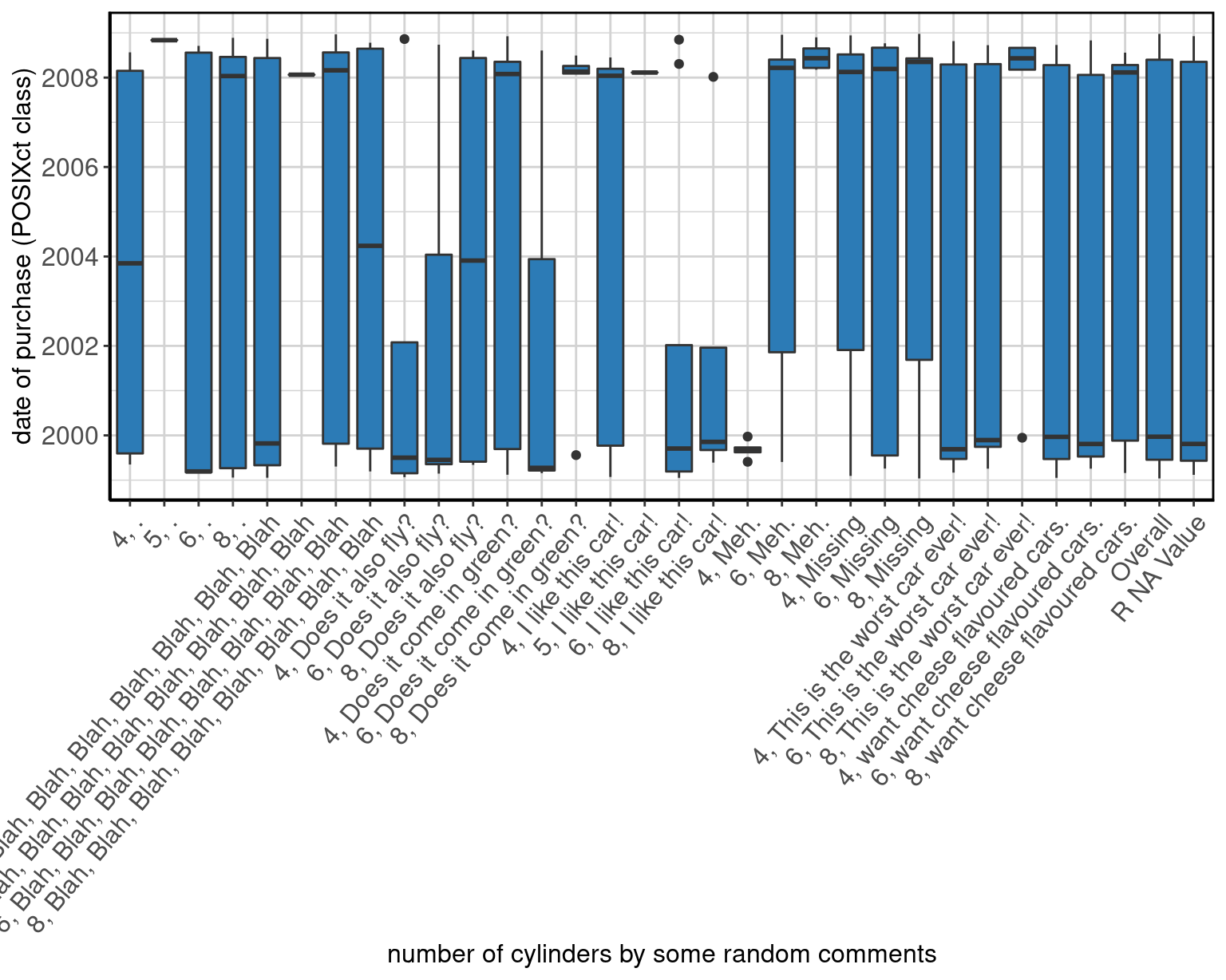
Figure 15: Stacked barplot of date of purchase (Date class) by number of cylinders by some random comments.
Difftime
For a difftime variable x, we need to specify x, the data, and difftime_units.
rdifftimeSummaryExample <- data_summary(x = "rdifftime", data = mpg, difftime_units = "weeks")Show method to output table and plot
show(rdifftimeSummaryExample)##
## 1
## Label
## 1 some random numbers that are generated from a normal distrubtion with mean = 10 and sd = 5, and then converted to weeks
## N P NA Mean S Dev Med MAD 25th P 75th P
## 1 184 21.37 9.76 weeks 5.07 weeks 9.6 weeks 5.12 weeks 6.11 weeks 13.05 weeks
## IQR Min Max
## 1 6.79 weeks 0 weeks 23.49 weeks
Output the summary table
data_summary_table(rdifftimeSummaryExample)##
## 1
## Label
## 1 some random numbers that are generated from a normal distrubtion with mean = 10 and sd = 5, and then converted to weeks
## N P NA Mean S Dev Med MAD 25th P 75th P
## 1 184 21.37 9.76 weeks 5.07 weeks 9.6 weeks 5.12 weeks 6.11 weeks 13.05 weeks
## IQR Min Max
## 1 6.79 weeks 0 weeks 23.49 weeksOutput the plot
data_summary_plot(rdifftimeSummaryExample)
Generate knitr friendly summary table
make_kable_output(rdifftimeSummaryExample)| Label | N | P NA | Mean | S Dev | Med | MAD | 25th P | 75th P | IQR | Min | Max | |
|---|---|---|---|---|---|---|---|---|---|---|---|---|
| some random numbers that are generated from a normal distrubtion with mean = 10 and sd = 5, and then converted to weeks | 184 | 21.37 | 9.76 weeks | 5.07 weeks | 9.6 weeks | 5.12 weeks | 6.11 weeks | 13.05 weeks | 6.79 weeks | 0 weeks | 23.49 weeks |
Generate knitr friendly output
make_complete_output(rdifftimeSummaryExample)| Label | N | P NA | Mean | S Dev | Med | MAD | 25th P | 75th P | IQR | Min | Max | |
|---|---|---|---|---|---|---|---|---|---|---|---|---|
| some random numbers that are generated from a normal distrubtion with mean = 10 and sd = 5, and then converted to weeks | 184 | 21.37 | 9.76 weeks | 5.07 weeks | 9.6 weeks | 5.12 weeks | 6.11 weeks | 13.05 weeks | 6.79 weeks | 0 weeks | 23.49 weeks |
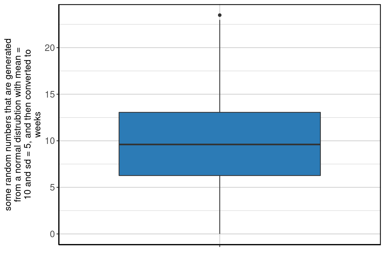
Figure 16: Stacked barplot of some random numbers that are generated from a normal distrubtion with mean = 10 and sd = 5, and then converted to weeks.
Difftime By
For a date variable with by, we need to specify x, a by variable, the data, and difftime_units.
rdifftimeByDrvSummaryExample <- data_summary(x = "rdifftime", by = "drv", data = mpg, difftime_units = "weeks")Show method to output table and plot
show(rdifftimeByDrvSummaryExample)## drive type
## 1 front-wheel drive
## 2 rear wheel drive
## 3 4wd
## 4 Overall
## Label
## 1 some random numbers that are generated from a normal distrubtion with mean = 10 and sd = 5, and then converted to weeks
## 2 some random numbers that are generated from a normal distrubtion with mean = 10 and sd = 5, and then converted to weeks
## 3 some random numbers that are generated from a normal distrubtion with mean = 10 and sd = 5, and then converted to weeks
## 4 some random numbers that are generated from a normal distrubtion with mean = 10 and sd = 5, and then converted to weeks
## N P NA Mean S Dev Med MAD 25th P
## 1 86 18.87 10.57 weeks 5.24 weeks 10.79 weeks 4.80 weeks 6.59 weeks
## 2 19 24.00 8.43 weeks 5.17 weeks 8.57 weeks 5.74 weeks 4.70 weeks
## 3 79 23.30 9.19 weeks 4.77 weeks 9.02 weeks 4.77 weeks 6.11 weeks
## 4 184 21.37 9.76 weeks 5.07 weeks 9.60 weeks 5.12 weeks 6.11 weeks
## 75th P IQR Min Max
## 1 13.57 weeks 6.87 weeks 0 weeks 23.49 weeks
## 2 12.72 weeks 7.27 weeks 0 weeks 19.07 weeks
## 3 12.58 weeks 6.15 weeks 0 weeks 21.71 weeks
## 4 13.05 weeks 6.79 weeks 0 weeks 23.49 weeks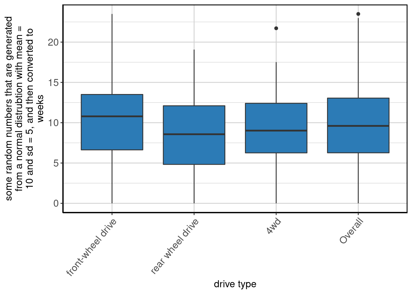
Output the summary table
data_summary_table(rdifftimeByDrvSummaryExample)## drive type
## 1 front-wheel drive
## 2 rear wheel drive
## 3 4wd
## 4 Overall
## Label
## 1 some random numbers that are generated from a normal distrubtion with mean = 10 and sd = 5, and then converted to weeks
## 2 some random numbers that are generated from a normal distrubtion with mean = 10 and sd = 5, and then converted to weeks
## 3 some random numbers that are generated from a normal distrubtion with mean = 10 and sd = 5, and then converted to weeks
## 4 some random numbers that are generated from a normal distrubtion with mean = 10 and sd = 5, and then converted to weeks
## N P NA Mean S Dev Med MAD 25th P
## 1 86 18.87 10.57 weeks 5.24 weeks 10.79 weeks 4.80 weeks 6.59 weeks
## 2 19 24.00 8.43 weeks 5.17 weeks 8.57 weeks 5.74 weeks 4.70 weeks
## 3 79 23.30 9.19 weeks 4.77 weeks 9.02 weeks 4.77 weeks 6.11 weeks
## 4 184 21.37 9.76 weeks 5.07 weeks 9.60 weeks 5.12 weeks 6.11 weeks
## 75th P IQR Min Max
## 1 13.57 weeks 6.87 weeks 0 weeks 23.49 weeks
## 2 12.72 weeks 7.27 weeks 0 weeks 19.07 weeks
## 3 12.58 weeks 6.15 weeks 0 weeks 21.71 weeks
## 4 13.05 weeks 6.79 weeks 0 weeks 23.49 weeksOutput the plot
data_summary_plot(rdifftimeByDrvSummaryExample)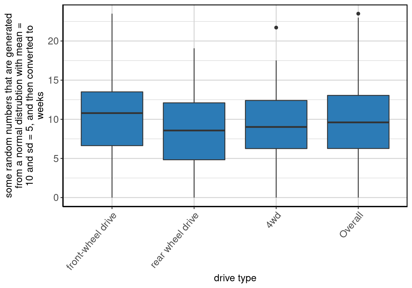
Generate a knitr friendly summary table
make_kable_output(rdifftimeByDrvSummaryExample)| drive type | Label | N | P NA | Mean | S Dev | Med | MAD | 25th P | 75th P | IQR | Min | Max |
|---|---|---|---|---|---|---|---|---|---|---|---|---|
| front-wheel drive | some random numbers that are generated from a normal distrubtion with mean = 10 and sd = 5, and then converted to weeks | 86 | 18.87 | 10.57 weeks | 5.24 weeks | 10.79 weeks | 4.80 weeks | 6.59 weeks | 13.57 weeks | 6.87 weeks | 0 weeks | 23.49 weeks |
| rear wheel drive | some random numbers that are generated from a normal distrubtion with mean = 10 and sd = 5, and then converted to weeks | 19 | 24.00 | 8.43 weeks | 5.17 weeks | 8.57 weeks | 5.74 weeks | 4.70 weeks | 12.72 weeks | 7.27 weeks | 0 weeks | 19.07 weeks |
| 4wd | some random numbers that are generated from a normal distrubtion with mean = 10 and sd = 5, and then converted to weeks | 79 | 23.30 | 9.19 weeks | 4.77 weeks | 9.02 weeks | 4.77 weeks | 6.11 weeks | 12.58 weeks | 6.15 weeks | 0 weeks | 21.71 weeks |
| Overall | some random numbers that are generated from a normal distrubtion with mean = 10 and sd = 5, and then converted to weeks | 184 | 21.37 | 9.76 weeks | 5.07 weeks | 9.60 weeks | 5.12 weeks | 6.11 weeks | 13.05 weeks | 6.79 weeks | 0 weeks | 23.49 weeks |
Generate knitr friendly output
make_complete_output(rdifftimeByDrvSummaryExample)| drive type | Label | N | P NA | Mean | S Dev | Med | MAD | 25th P | 75th P | IQR | Min | Max |
|---|---|---|---|---|---|---|---|---|---|---|---|---|
| front-wheel drive | some random numbers that are generated from a normal distrubtion with mean = 10 and sd = 5, and then converted to weeks | 86 | 18.87 | 10.57 weeks | 5.24 weeks | 10.79 weeks | 4.80 weeks | 6.59 weeks | 13.57 weeks | 6.87 weeks | 0 weeks | 23.49 weeks |
| rear wheel drive | some random numbers that are generated from a normal distrubtion with mean = 10 and sd = 5, and then converted to weeks | 19 | 24.00 | 8.43 weeks | 5.17 weeks | 8.57 weeks | 5.74 weeks | 4.70 weeks | 12.72 weeks | 7.27 weeks | 0 weeks | 19.07 weeks |
| 4wd | some random numbers that are generated from a normal distrubtion with mean = 10 and sd = 5, and then converted to weeks | 79 | 23.30 | 9.19 weeks | 4.77 weeks | 9.02 weeks | 4.77 weeks | 6.11 weeks | 12.58 weeks | 6.15 weeks | 0 weeks | 21.71 weeks |
| Overall | some random numbers that are generated from a normal distrubtion with mean = 10 and sd = 5, and then converted to weeks | 184 | 21.37 | 9.76 weeks | 5.07 weeks | 9.60 weeks | 5.12 weeks | 6.11 weeks | 13.05 weeks | 6.79 weeks | 0 weeks | 23.49 weeks |

Figure 17: Stacked barplot of some random numbers that are generated from a normal distrubtion with mean = 10 and sd = 5, and then converted to weeks by drive type.
Difftime By By
For a date variable with two or more by variables, we need to specify x, the by variables as a character string, the data, and difftime_units.
rdifftimeByDrvBypartySummaryExample <- data_summary(x = "rdifftime", by = c("drv", "party"), data = mpg, difftime_units = "weeks")Show method to output table and plot
show(rdifftimeByDrvBypartySummaryExample)## drive type by some random political parties
## 1 front-wheel drive, republican
## 2 rear wheel drive, republican
## 3 4wd, republican
## 4 front-wheel drive, democrat
## 5 rear wheel drive, democrat
## 6 4wd, democrat
## 7 front-wheel drive, independent
## 8 rear wheel drive, independent
## 9 4wd, independent
## 10 Overall
## 11 R NA Value
## Label
## 1 some random numbers that are generated from a normal distrubtion with mean = 10 and sd = 5, and then converted to weeks
## 2 some random numbers that are generated from a normal distrubtion with mean = 10 and sd = 5, and then converted to weeks
## 3 some random numbers that are generated from a normal distrubtion with mean = 10 and sd = 5, and then converted to weeks
## 4 some random numbers that are generated from a normal distrubtion with mean = 10 and sd = 5, and then converted to weeks
## 5 some random numbers that are generated from a normal distrubtion with mean = 10 and sd = 5, and then converted to weeks
## 6 some random numbers that are generated from a normal distrubtion with mean = 10 and sd = 5, and then converted to weeks
## 7 some random numbers that are generated from a normal distrubtion with mean = 10 and sd = 5, and then converted to weeks
## 8 some random numbers that are generated from a normal distrubtion with mean = 10 and sd = 5, and then converted to weeks
## 9 some random numbers that are generated from a normal distrubtion with mean = 10 and sd = 5, and then converted to weeks
## 10 some random numbers that are generated from a normal distrubtion with mean = 10 and sd = 5, and then converted to weeks
## 11 some random numbers that are generated from a normal distrubtion with mean = 10 and sd = 5, and then converted to weeks
## N P NA Mean S Dev Med MAD 25th P
## 1 18 30.77 8.95 weeks 6.26 weeks 9.97 weeks 5.64 weeks 4.95 weeks
## 2 4 0.00 8.75 weeks 4.34 weeks 8.31 weeks 4.84 weeks 4.96 weeks
## 3 23 11.54 10.07 weeks 6.02 weeks 11.25 weeks 6.73 weeks 4.81 weeks
## 4 17 5.56 11.37 weeks 4.11 weeks 12.03 weeks 4.84 weeks 7.55 weeks
## 5 5 16.67 8.26 weeks 3.99 weeks 9.35 weeks 5.25 weeks 4.70 weeks
## 6 30 18.92 8.31 weeks 4.50 weeks 7.60 weeks 5.60 weeks 6.41 weeks
## 7 26 18.75 10.75 weeks 4.96 weeks 10.31 weeks 4.84 weeks 5.99 weeks
## 8 6 14.29 8.80 weeks 5.07 weeks 8.18 weeks 5.40 weeks 5.44 weeks
## 9 15 34.78 9.86 weeks 4.04 weeks 9.58 weeks 5.87 weeks 5.61 weeks
## 10 184 21.37 9.76 weeks 5.07 weeks 9.60 weeks 5.12 weeks 6.11 weeks
## 11 40 27.27 10.08 weeks 5.38 weeks 10.06 weeks 4.12 weeks 6.76 weeks
## 75th P IQR Min Max
## 1 11.98 weeks 6.63 weeks 0.00 weeks 23.49 weeks
## 2 11.48 weeks 6.87 weeks 4.96 weeks 13.41 weeks
## 3 15.45 weeks 9.23 weeks 0.00 weeks 21.71 weeks
## 4 13.88 weeks 6.32 weeks 5.05 weeks 18.28 weeks
## 5 10.78 weeks 6.08 weeks 3.57 weeks 12.89 weeks
## 6 11.90 weeks 5.46 weeks 0.00 weeks 16.25 weeks
## 7 13.57 weeks 6.80 weeks 2.95 weeks 21.65 weeks
## 8 12.72 weeks 5.66 weeks 2.04 weeks 16.22 weeks
## 9 13.65 weeks 6.94 weeks 4.33 weeks 15.38 weeks
## 10 13.05 weeks 6.79 weeks 0.00 weeks 23.49 weeks
## 11 12.27 weeks 5.46 weeks 0.00 weeks 22.98 weeks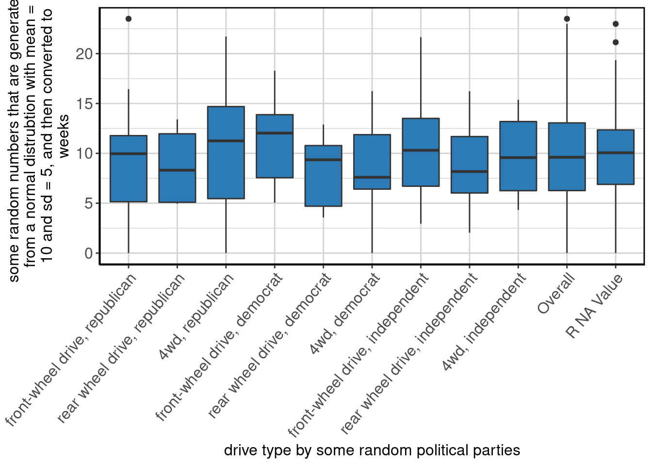
Output the summary table
data_summary_table(rdifftimeByDrvBypartySummaryExample)## drive type by some random political parties
## 1 front-wheel drive, republican
## 2 rear wheel drive, republican
## 3 4wd, republican
## 4 front-wheel drive, democrat
## 5 rear wheel drive, democrat
## 6 4wd, democrat
## 7 front-wheel drive, independent
## 8 rear wheel drive, independent
## 9 4wd, independent
## 10 Overall
## 11 R NA Value
## Label
## 1 some random numbers that are generated from a normal distrubtion with mean = 10 and sd = 5, and then converted to weeks
## 2 some random numbers that are generated from a normal distrubtion with mean = 10 and sd = 5, and then converted to weeks
## 3 some random numbers that are generated from a normal distrubtion with mean = 10 and sd = 5, and then converted to weeks
## 4 some random numbers that are generated from a normal distrubtion with mean = 10 and sd = 5, and then converted to weeks
## 5 some random numbers that are generated from a normal distrubtion with mean = 10 and sd = 5, and then converted to weeks
## 6 some random numbers that are generated from a normal distrubtion with mean = 10 and sd = 5, and then converted to weeks
## 7 some random numbers that are generated from a normal distrubtion with mean = 10 and sd = 5, and then converted to weeks
## 8 some random numbers that are generated from a normal distrubtion with mean = 10 and sd = 5, and then converted to weeks
## 9 some random numbers that are generated from a normal distrubtion with mean = 10 and sd = 5, and then converted to weeks
## 10 some random numbers that are generated from a normal distrubtion with mean = 10 and sd = 5, and then converted to weeks
## 11 some random numbers that are generated from a normal distrubtion with mean = 10 and sd = 5, and then converted to weeks
## N P NA Mean S Dev Med MAD 25th P
## 1 18 30.77 8.95 weeks 6.26 weeks 9.97 weeks 5.64 weeks 4.95 weeks
## 2 4 0.00 8.75 weeks 4.34 weeks 8.31 weeks 4.84 weeks 4.96 weeks
## 3 23 11.54 10.07 weeks 6.02 weeks 11.25 weeks 6.73 weeks 4.81 weeks
## 4 17 5.56 11.37 weeks 4.11 weeks 12.03 weeks 4.84 weeks 7.55 weeks
## 5 5 16.67 8.26 weeks 3.99 weeks 9.35 weeks 5.25 weeks 4.70 weeks
## 6 30 18.92 8.31 weeks 4.50 weeks 7.60 weeks 5.60 weeks 6.41 weeks
## 7 26 18.75 10.75 weeks 4.96 weeks 10.31 weeks 4.84 weeks 5.99 weeks
## 8 6 14.29 8.80 weeks 5.07 weeks 8.18 weeks 5.40 weeks 5.44 weeks
## 9 15 34.78 9.86 weeks 4.04 weeks 9.58 weeks 5.87 weeks 5.61 weeks
## 10 184 21.37 9.76 weeks 5.07 weeks 9.60 weeks 5.12 weeks 6.11 weeks
## 11 40 27.27 10.08 weeks 5.38 weeks 10.06 weeks 4.12 weeks 6.76 weeks
## 75th P IQR Min Max
## 1 11.98 weeks 6.63 weeks 0.00 weeks 23.49 weeks
## 2 11.48 weeks 6.87 weeks 4.96 weeks 13.41 weeks
## 3 15.45 weeks 9.23 weeks 0.00 weeks 21.71 weeks
## 4 13.88 weeks 6.32 weeks 5.05 weeks 18.28 weeks
## 5 10.78 weeks 6.08 weeks 3.57 weeks 12.89 weeks
## 6 11.90 weeks 5.46 weeks 0.00 weeks 16.25 weeks
## 7 13.57 weeks 6.80 weeks 2.95 weeks 21.65 weeks
## 8 12.72 weeks 5.66 weeks 2.04 weeks 16.22 weeks
## 9 13.65 weeks 6.94 weeks 4.33 weeks 15.38 weeks
## 10 13.05 weeks 6.79 weeks 0.00 weeks 23.49 weeks
## 11 12.27 weeks 5.46 weeks 0.00 weeks 22.98 weeksOutput the plot
data_summary_plot(rdifftimeByDrvBypartySummaryExample)
Generate a knitr friendly summary table
make_kable_output(rdifftimeByDrvBypartySummaryExample)| drive type by some random political parties | Label | N | P NA | Mean | S Dev | Med | MAD | 25th P | 75th P | IQR | Min | Max |
|---|---|---|---|---|---|---|---|---|---|---|---|---|
| front-wheel drive, republican | some random numbers that are generated from a normal distrubtion with mean = 10 and sd = 5, and then converted to weeks | 18 | 30.77 | 8.95 weeks | 6.26 weeks | 9.97 weeks | 5.64 weeks | 4.95 weeks | 11.98 weeks | 6.63 weeks | 0.00 weeks | 23.49 weeks |
| rear wheel drive, republican | some random numbers that are generated from a normal distrubtion with mean = 10 and sd = 5, and then converted to weeks | 4 | 0.00 | 8.75 weeks | 4.34 weeks | 8.31 weeks | 4.84 weeks | 4.96 weeks | 11.48 weeks | 6.87 weeks | 4.96 weeks | 13.41 weeks |
| 4wd, republican | some random numbers that are generated from a normal distrubtion with mean = 10 and sd = 5, and then converted to weeks | 23 | 11.54 | 10.07 weeks | 6.02 weeks | 11.25 weeks | 6.73 weeks | 4.81 weeks | 15.45 weeks | 9.23 weeks | 0.00 weeks | 21.71 weeks |
| front-wheel drive, democrat | some random numbers that are generated from a normal distrubtion with mean = 10 and sd = 5, and then converted to weeks | 17 | 5.56 | 11.37 weeks | 4.11 weeks | 12.03 weeks | 4.84 weeks | 7.55 weeks | 13.88 weeks | 6.32 weeks | 5.05 weeks | 18.28 weeks |
| rear wheel drive, democrat | some random numbers that are generated from a normal distrubtion with mean = 10 and sd = 5, and then converted to weeks | 5 | 16.67 | 8.26 weeks | 3.99 weeks | 9.35 weeks | 5.25 weeks | 4.70 weeks | 10.78 weeks | 6.08 weeks | 3.57 weeks | 12.89 weeks |
| 4wd, democrat | some random numbers that are generated from a normal distrubtion with mean = 10 and sd = 5, and then converted to weeks | 30 | 18.92 | 8.31 weeks | 4.50 weeks | 7.60 weeks | 5.60 weeks | 6.41 weeks | 11.90 weeks | 5.46 weeks | 0.00 weeks | 16.25 weeks |
| front-wheel drive, independent | some random numbers that are generated from a normal distrubtion with mean = 10 and sd = 5, and then converted to weeks | 26 | 18.75 | 10.75 weeks | 4.96 weeks | 10.31 weeks | 4.84 weeks | 5.99 weeks | 13.57 weeks | 6.80 weeks | 2.95 weeks | 21.65 weeks |
| rear wheel drive, independent | some random numbers that are generated from a normal distrubtion with mean = 10 and sd = 5, and then converted to weeks | 6 | 14.29 | 8.80 weeks | 5.07 weeks | 8.18 weeks | 5.40 weeks | 5.44 weeks | 12.72 weeks | 5.66 weeks | 2.04 weeks | 16.22 weeks |
| 4wd, independent | some random numbers that are generated from a normal distrubtion with mean = 10 and sd = 5, and then converted to weeks | 15 | 34.78 | 9.86 weeks | 4.04 weeks | 9.58 weeks | 5.87 weeks | 5.61 weeks | 13.65 weeks | 6.94 weeks | 4.33 weeks | 15.38 weeks |
| Overall | some random numbers that are generated from a normal distrubtion with mean = 10 and sd = 5, and then converted to weeks | 184 | 21.37 | 9.76 weeks | 5.07 weeks | 9.60 weeks | 5.12 weeks | 6.11 weeks | 13.05 weeks | 6.79 weeks | 0.00 weeks | 23.49 weeks |
| R NA Value | some random numbers that are generated from a normal distrubtion with mean = 10 and sd = 5, and then converted to weeks | 40 | 27.27 | 10.08 weeks | 5.38 weeks | 10.06 weeks | 4.12 weeks | 6.76 weeks | 12.27 weeks | 5.46 weeks | 0.00 weeks | 22.98 weeks |
Generate knitr friendly output
make_complete_output(rdifftimeByDrvBypartySummaryExample)| drive type by some random political parties | Label | N | P NA | Mean | S Dev | Med | MAD | 25th P | 75th P | IQR | Min | Max |
|---|---|---|---|---|---|---|---|---|---|---|---|---|
| front-wheel drive, republican | some random numbers that are generated from a normal distrubtion with mean = 10 and sd = 5, and then converted to weeks | 18 | 30.77 | 8.95 weeks | 6.26 weeks | 9.97 weeks | 5.64 weeks | 4.95 weeks | 11.98 weeks | 6.63 weeks | 0.00 weeks | 23.49 weeks |
| rear wheel drive, republican | some random numbers that are generated from a normal distrubtion with mean = 10 and sd = 5, and then converted to weeks | 4 | 0.00 | 8.75 weeks | 4.34 weeks | 8.31 weeks | 4.84 weeks | 4.96 weeks | 11.48 weeks | 6.87 weeks | 4.96 weeks | 13.41 weeks |
| 4wd, republican | some random numbers that are generated from a normal distrubtion with mean = 10 and sd = 5, and then converted to weeks | 23 | 11.54 | 10.07 weeks | 6.02 weeks | 11.25 weeks | 6.73 weeks | 4.81 weeks | 15.45 weeks | 9.23 weeks | 0.00 weeks | 21.71 weeks |
| front-wheel drive, democrat | some random numbers that are generated from a normal distrubtion with mean = 10 and sd = 5, and then converted to weeks | 17 | 5.56 | 11.37 weeks | 4.11 weeks | 12.03 weeks | 4.84 weeks | 7.55 weeks | 13.88 weeks | 6.32 weeks | 5.05 weeks | 18.28 weeks |
| rear wheel drive, democrat | some random numbers that are generated from a normal distrubtion with mean = 10 and sd = 5, and then converted to weeks | 5 | 16.67 | 8.26 weeks | 3.99 weeks | 9.35 weeks | 5.25 weeks | 4.70 weeks | 10.78 weeks | 6.08 weeks | 3.57 weeks | 12.89 weeks |
| 4wd, democrat | some random numbers that are generated from a normal distrubtion with mean = 10 and sd = 5, and then converted to weeks | 30 | 18.92 | 8.31 weeks | 4.50 weeks | 7.60 weeks | 5.60 weeks | 6.41 weeks | 11.90 weeks | 5.46 weeks | 0.00 weeks | 16.25 weeks |
| front-wheel drive, independent | some random numbers that are generated from a normal distrubtion with mean = 10 and sd = 5, and then converted to weeks | 26 | 18.75 | 10.75 weeks | 4.96 weeks | 10.31 weeks | 4.84 weeks | 5.99 weeks | 13.57 weeks | 6.80 weeks | 2.95 weeks | 21.65 weeks |
| rear wheel drive, independent | some random numbers that are generated from a normal distrubtion with mean = 10 and sd = 5, and then converted to weeks | 6 | 14.29 | 8.80 weeks | 5.07 weeks | 8.18 weeks | 5.40 weeks | 5.44 weeks | 12.72 weeks | 5.66 weeks | 2.04 weeks | 16.22 weeks |
| 4wd, independent | some random numbers that are generated from a normal distrubtion with mean = 10 and sd = 5, and then converted to weeks | 15 | 34.78 | 9.86 weeks | 4.04 weeks | 9.58 weeks | 5.87 weeks | 5.61 weeks | 13.65 weeks | 6.94 weeks | 4.33 weeks | 15.38 weeks |
| Overall | some random numbers that are generated from a normal distrubtion with mean = 10 and sd = 5, and then converted to weeks | 184 | 21.37 | 9.76 weeks | 5.07 weeks | 9.60 weeks | 5.12 weeks | 6.11 weeks | 13.05 weeks | 6.79 weeks | 0.00 weeks | 23.49 weeks |
| R NA Value | some random numbers that are generated from a normal distrubtion with mean = 10 and sd = 5, and then converted to weeks | 40 | 27.27 | 10.08 weeks | 5.38 weeks | 10.06 weeks | 4.12 weeks | 6.76 weeks | 12.27 weeks | 5.46 weeks | 0.00 weeks | 22.98 weeks |
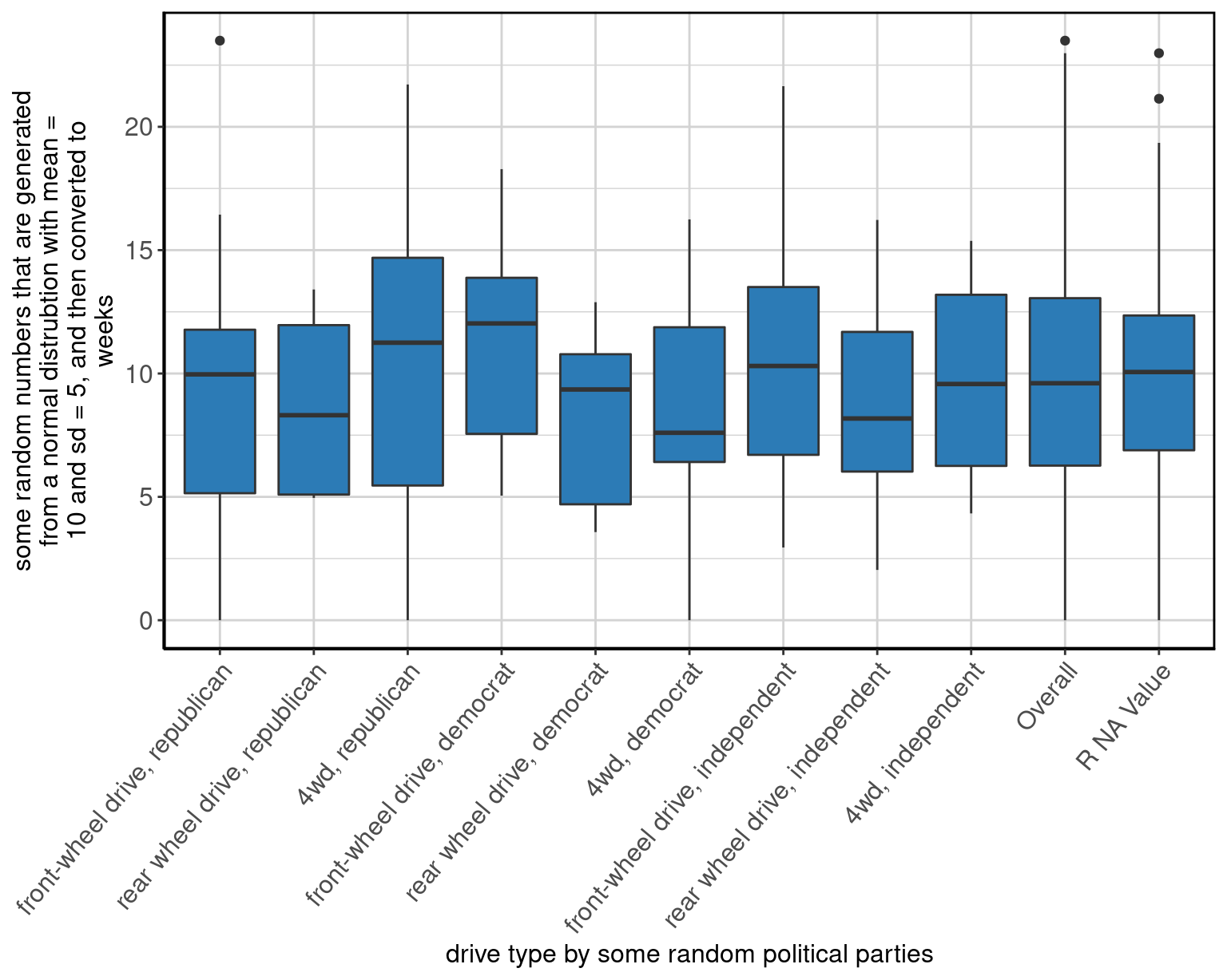
Figure 18: Stacked barplot of some random numbers that are generated from a normal distrubtion with mean = 10 and sd = 5, and then converted to weeks by drive type by some random political parties.
Data Summaries
Manufacturer
The results are in table 38 and figure 19.
manuSummary <- data_summary(x = "manu", data = mpg)

make_complete_output(manuSummary)| manufacturer | n (%) |
|---|---|
| audi | 18 (7.69%) |
| chevrolet | 19 (8.12%) |
| dodge | 37 (15.81%) |
| ford | 25 (10.68%) |
| honda | 9 (3.85%) |
| hyundai | 14 (5.98%) |
| jeep | 8 (3.42%) |
| land rover | 4 (1.71%) |
| lincoln | 3 (1.28%) |
| mercury | 4 (1.71%) |
| nissan | 13 (5.56%) |
| pontiac | 5 (2.14%) |
| subaru | 14 (5.98%) |
| toyota | 34 (14.53%) |
| volkswagen | 27 (11.54%) |
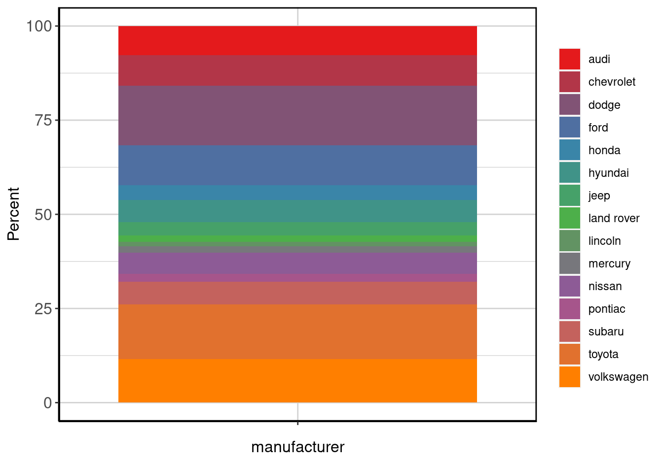
Figure 19: Stacked barplot of manufacturer.
Model Name
The results are in table 39 and figure 20.
modelSummary <- data_summary(x = "model", data = mpg)

make_complete_output(modelSummary)| model name | n (%) |
|---|---|
| 4runner 4wd | 6 (2.56%) |
| a4 | 7 (2.99%) |
| a4 quattro | 8 (3.42%) |
| a6 quattro | 3 (1.28%) |
| altima | 6 (2.56%) |
| c1500 suburban 2wd | 5 (2.14%) |
| camry | 7 (2.99%) |
| camry solara | 7 (2.99%) |
| caravan 2wd | 11 (4.7%) |
| civic | 9 (3.85%) |
| corolla | 5 (2.14%) |
| corvette | 5 (2.14%) |
| dakota pickup 4wd | 9 (3.85%) |
| durango 4wd | 7 (2.99%) |
| expedition 2wd | 3 (1.28%) |
| explorer 4wd | 6 (2.56%) |
| f150 pickup 4wd | 7 (2.99%) |
| forester awd | 6 (2.56%) |
| grand cherokee 4wd | 8 (3.42%) |
| grand prix | 5 (2.14%) |
| gti | 5 (2.14%) |
| impreza awd | 8 (3.42%) |
| jetta | 9 (3.85%) |
| k1500 tahoe 4wd | 4 (1.71%) |
| land cruiser wagon 4wd | 2 (0.85%) |
| malibu | 5 (2.14%) |
| maxima | 3 (1.28%) |
| mountaineer 4wd | 4 (1.71%) |
| mustang | 9 (3.85%) |
| navigator 2wd | 3 (1.28%) |
| new beetle | 6 (2.56%) |
| passat | 7 (2.99%) |
| pathfinder 4wd | 4 (1.71%) |
| ram 1500 pickup 4wd | 10 (4.27%) |
| range rover | 4 (1.71%) |
| sonata | 7 (2.99%) |
| tiburon | 7 (2.99%) |
| toyota tacoma 4wd | 7 (2.99%) |
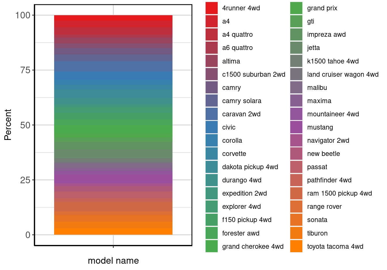
Figure 20: Stacked barplot of model name.
Engine Displacement (Litres)
The results are in table 40 and figure 21.
displSummary <- data_summary(x = "displ", data = mpg)

make_complete_output(displSummary)| Label | N | P NA | Mean | S Dev | Med | MAD | 25th P | 75th P | IQR | Min | Max | |
|---|---|---|---|---|---|---|---|---|---|---|---|---|
| engine displacement, in litres | 234 | 0 | 3.47 | 1.29 | 3.3 | 1.33 | 2.4 | 4.6 | 2.2 | 1.6 | 7 |
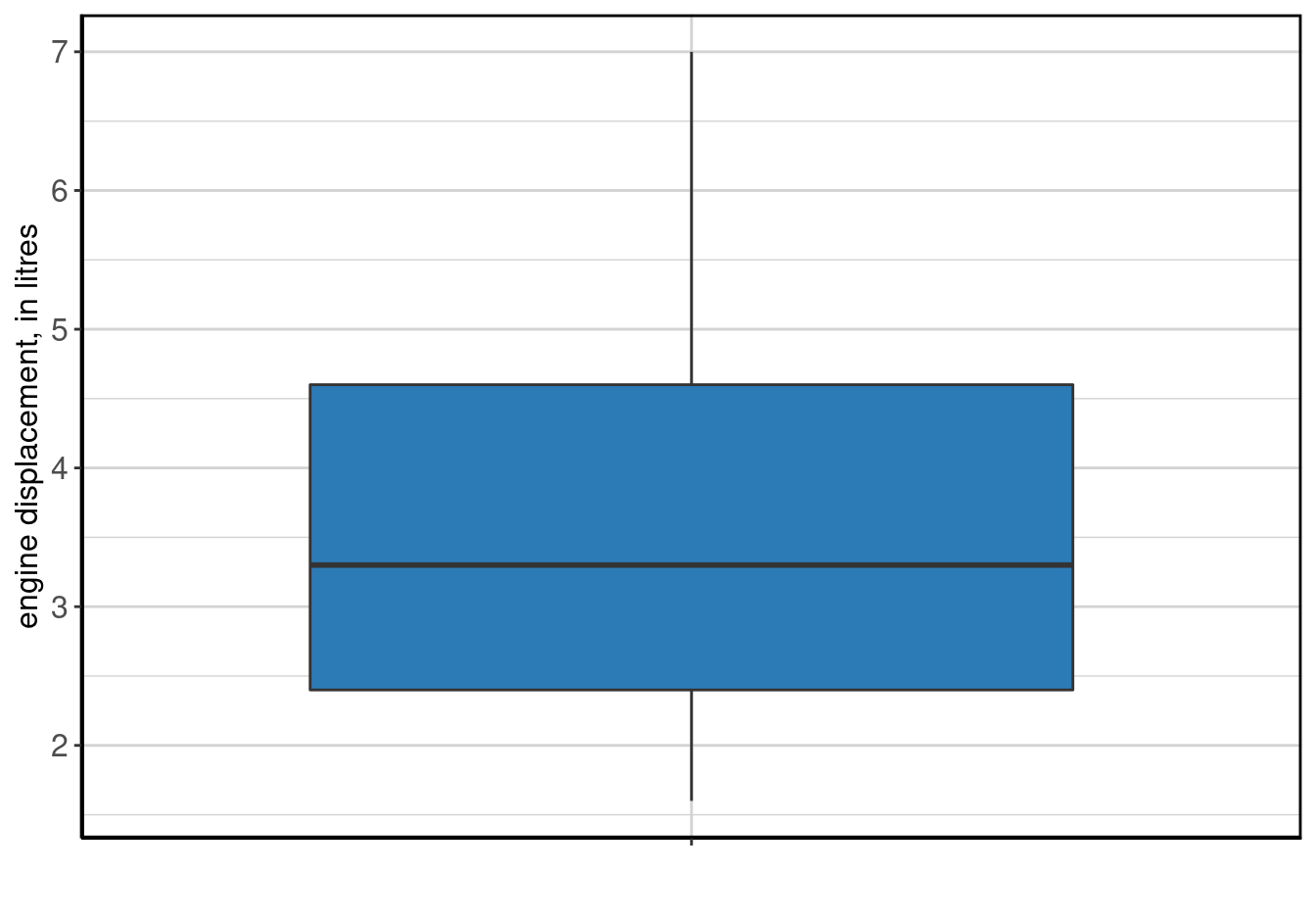
Figure 21: Boxplot of engine displacement, in litres.
Year of Manufacture
The results are in table 41 and figure 22.
yearSummary <- data_summary(x = "year", data = mpg)

make_complete_output(yearSummary)| year of manufacture | n (%) |
|---|---|
| 1999 | 117 (50%) |
| 2008 | 117 (50%) |
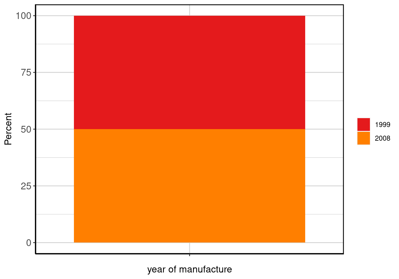
Figure 22: Stacked barplot of year of manufacture.
Date of Purchase
The results are in table 42 and figure 23.
dpSummary <- data_summary(x = "dp", data = mpg[which(mpg$dp != "1000-05-02" | is.na(mpg$dp)), ], difftime_units = "weeks")

make_complete_output(dpSummary)| Label | N | P NA | Mean | S Dev | Med | MAD | 25th P | 75th P | IQR | Min | Max | |
|---|---|---|---|---|---|---|---|---|---|---|---|---|
| date of purchase (Date class) | 213 | 8.58 | 2003-12-21 | 236.59 weeks | 1999-12-24 | 74.98 weeks | 1999-07-14 | 2008-09-01 | 476.7143 weeks | 1999-01-04 | 2008-12-23 |

Figure 23: Boxplot of date of purchase (Date class).
Number of Cylinders
The results are in table 43 and figure 24.
cylSummary <- data_summary(x = "cyl", data = mpg)

make_complete_output(cylSummary)| number of cylinders | n (%) |
|---|---|
| 4 | 81 (34.62%) |
| 5 | 4 (1.71%) |
| 6 | 79 (33.76%) |
| 8 | 70 (29.91%) |

Figure 24: Stacked barplot of number of cylinders.
Type of Transmission
The results are in table 44 and figure 25.
transSummary <- data_summary(x = "trans", data = mpg)

make_complete_output(transSummary)| type of transmission | n (%) |
|---|---|
| auto(av) | 5 (2.14%) |
| auto(l3) | 2 (0.85%) |
| auto(l4) | 83 (35.47%) |
| auto(l5) | 39 (16.67%) |
| auto(l6) | 6 (2.56%) |
| auto(s4) | 3 (1.28%) |
| auto(s5) | 3 (1.28%) |
| auto(s6) | 16 (6.84%) |
| manual(m5) | 58 (24.79%) |
| manual(m6) | 19 (8.12%) |
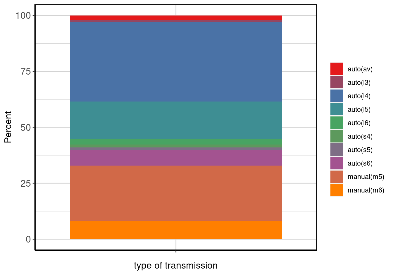
Figure 25: Stacked barplot of type of transmission.
Drive Type
The results are in table 45 and figure 26.
drvSummary <- data_summary(x = "drv", data = mpg)

make_complete_output(drvSummary)| drive type | n (%) |
|---|---|
| front-wheel drive | 106 (45.3%) |
| rear wheel drive | 25 (10.68%) |
| 4wd | 103 (44.02%) |
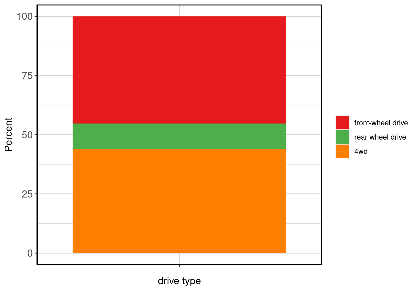
Figure 26: Stacked barplot of drive type.
City MPG
The results are in table 46 and figure 27.
ctySummary <- data_summary(x = "cty", data = mpg)

make_complete_output(ctySummary)| Label | N | P NA | Mean | S Dev | Med | MAD | 25th P | 75th P | IQR | Min | Max | |
|---|---|---|---|---|---|---|---|---|---|---|---|---|
| city miles per gallon | 234 | 0 | 16.86 | 4.26 | 17 | 4.45 | 14 | 19 | 5 | 9 | 35 |

Figure 27: Boxplot of city miles per gallon.
Highway MPG
The results are in table 47 and figure 28.
hwySummary <- data_summary(x = "hwy", data = mpg)

make_complete_output(hwySummary)| Label | N | P NA | Mean | S Dev | Med | MAD | 25th P | 75th P | IQR | Min | Max | |
|---|---|---|---|---|---|---|---|---|---|---|---|---|
| highway miles per gallon | 234 | 0 | 23.44 | 5.95 | 24 | 7.41 | 18 | 27 | 9 | 12 | 44 |
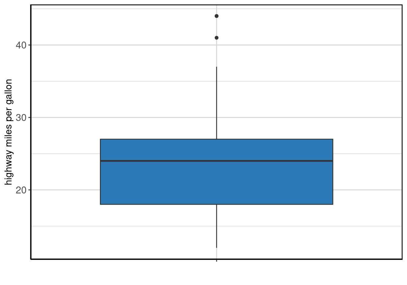
Figure 28: Boxplot of highway miles per gallon.
Fuel Type
The results are in table 48 and figure 29.
flSummary <- data_summary(x = "fl", data = mpg)

make_complete_output(flSummary)| fuel type | n (%) |
|---|---|
| c | 1 (0.43%) |
| d | 5 (2.14%) |
| e | 8 (3.42%) |
| p | 52 (22.22%) |
| r | 168 (71.79%) |
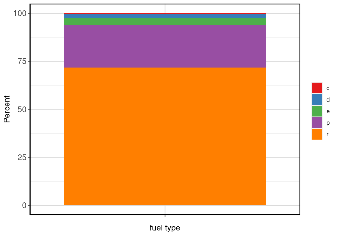
Figure 29: Stacked barplot of fuel type.
Type of Car
The results are in table 49 and figure 30.
classSummary <- data_summary(x = "class", data = mpg)

make_complete_output(classSummary)| type of car | n (%) |
|---|---|
| 2seater | 5 (2.14%) |
| compact | 47 (20.09%) |
| midsize | 41 (17.52%) |
| minivan | 11 (4.7%) |
| pickup | 33 (14.1%) |
| subcompact | 35 (14.96%) |
| suv | 62 (26.5%) |
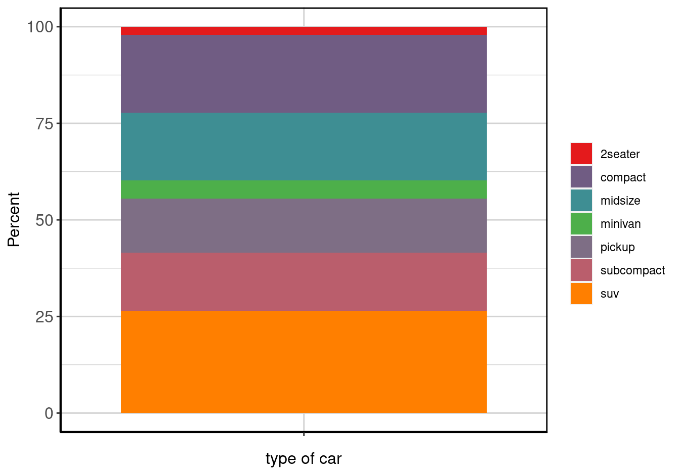
Figure 30: Stacked barplot of type of car.
Random Numbers
The results are in table 50 and figure 31.
rnSummary <- data_summary(x = "rn", data = mpg)

make_complete_output(rnSummary)| Label | N | P NA | Mean | S Dev | Med | MAD | 25th P | 75th P | IQR | Min | Max | |
|---|---|---|---|---|---|---|---|---|---|---|---|---|
| some random numbers that are generated from a normal distrubtion with mean = 10 and sd = 5 | 184 | 21.37 | 10.53 | 5.09 | 10.73 | 4.72 | 7.12 | 13.32 | 6.12 | -2.54 | 23.46 |
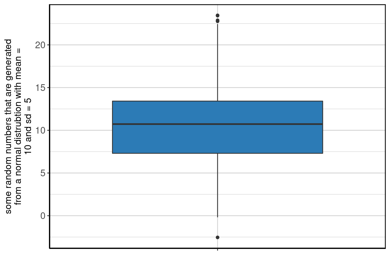
Figure 31: Boxplot of some random numbers that are generated from a normal distrubtion with mean = 10 and sd = 5.
Random Difference in Time
The results are in table 51 and figure 32.
rdifftimeSummary <- data_summary(x = "rdifftime", difftime_units = "weeks", data = mpg)

make_complete_output(rdifftimeSummary)| Label | N | P NA | Mean | S Dev | Med | MAD | 25th P | 75th P | IQR | Min | Max | |
|---|---|---|---|---|---|---|---|---|---|---|---|---|
| some random numbers that are generated from a normal distrubtion with mean = 10 and sd = 5, and then converted to weeks | 184 | 21.37 | 9.76 weeks | 5.07 weeks | 9.6 weeks | 5.12 weeks | 6.11 weeks | 13.05 weeks | 6.79 weeks | 0 weeks | 23.49 weeks |

Figure 32: Boxplot of some random numbers that are generated from a normal distrubtion with mean = 10 and sd = 5, and then converted to weeks.
Random Difference in Time Greater than 10
The results are in table 52 and figure 33.
logicalSummary <- data_summary(x = "logical", difftime_units = "weeks", data = mpg)

make_complete_output(logicalSummary)| some random numbers that are generated from a normal distrubtion with mean = 10 and sd = 5, and then converted to weeks, and then set to TRUE if the difference is greater than 10 | n (%) |
|---|---|
| FALSE | 96 (41.03%) |
| TRUE | 88 (37.61%) |
| R NA Value | 50 (21.37%) |
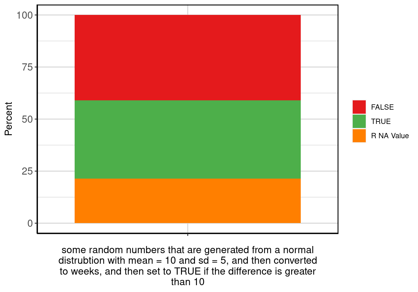
Figure 33: Boxplot of some random numbers that are generated from a normal distrubtion with mean = 10 and sd = 5, and then converted to weeks, and then set to TRUE if the difference is greater than 10.
Party
The results are in table 53 and figure 34.
partySummary <- data_summary(x = "party", data = mpg)

make_complete_output(partySummary)| some random political parties | n (%) |
|---|---|
| republican | 56 (23.93%) |
| democrat | 61 (26.07%) |
| independent | 62 (26.5%) |
| R NA Value | 55 (23.5%) |
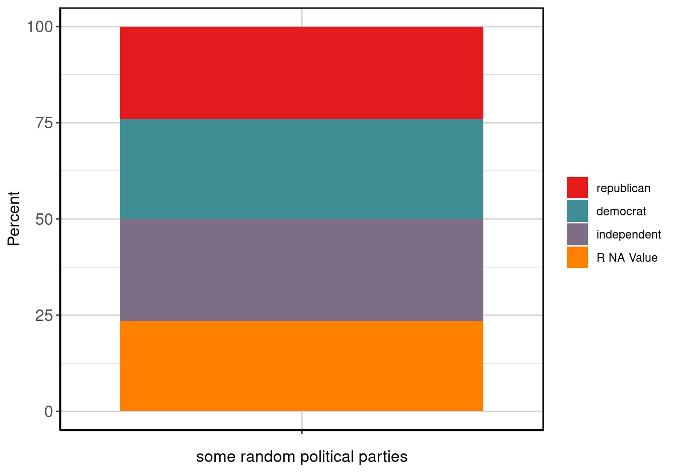
Figure 34: Stacked barplot of some random political parties.
All Missing
The results are in table 55 and figure 36.
missSummary <- data_summary(x = "miss", data = mpg)

make_complete_output(missSummary)| an all missing variable | n (%) |
|---|---|
| R NA Value | 234 (100%) |
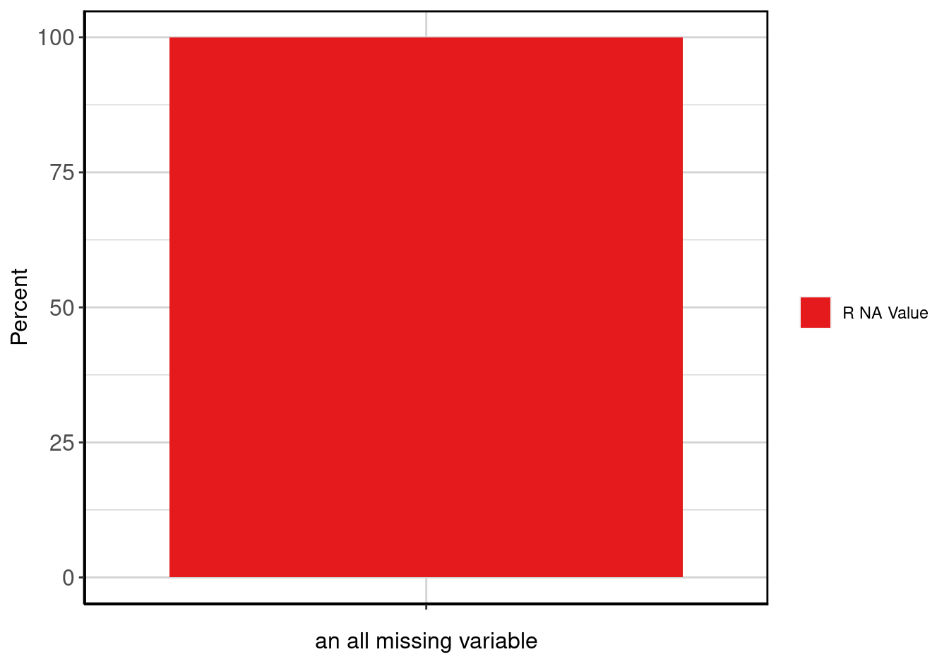
Figure 36: Stacked barplot of an all missing variable.
By Data Summaries
By Drive Type
Number of Cylinders by Drive Type
The results are in table 56 and figure 37.
cylByDrvSummary <- data_summary(x = "cyl", by = "drv", data = mpg)

make_complete_output(cylByDrvSummary)| number of cylinders | front-wheel drive | rear wheel drive | 4wd | Overall |
|---|---|---|---|---|
| 4 | 58 (54.72%) | 0 (0%) | 23 (22.33%) | 81 (34.62%) |
| 5 | 4 (3.77%) | 0 (0%) | 0 (0%) | 4 (1.71%) |
| 6 | 43 (40.57%) | 4 (16%) | 32 (31.07%) | 79 (33.76%) |
| 8 | 1 (0.94%) | 21 (84%) | 48 (46.6%) | 70 (29.91%) |
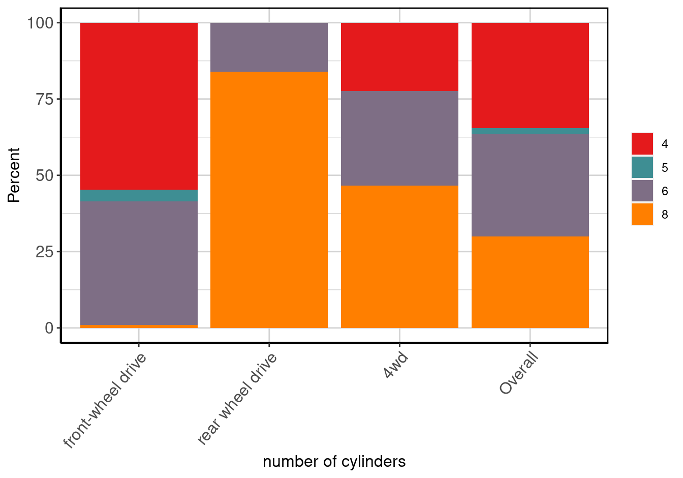
Figure 37: Stacked barplot of number of cylinders by drive type.
Date of Purchase by Drive Type
The results are in table 57 and figure 38.
dpByDrvSummary <- data_summary(x = "dp", by = "drv", data = mpg[which(mpg$dp != "1000-05-02" | is.na(mpg$dp)), ], difftime_units = "weeks")

make_complete_output(dpByDrvSummary)| drive type | Label | N | P NA | Mean | S Dev | Med | MAD | 25th P | 75th P | IQR | Min | Max |
|---|---|---|---|---|---|---|---|---|---|---|---|---|
| front-wheel drive | date of purchase (Date class) | 94 | 11.32 | 2003-06-08 | 235.20 weeks | 1999-11-21 | 60.47 weeks | 1999-07-03 | 2008-08-25 | 477.2857 weeks | 1999-01-07 | 2008-12-23 |
| rear wheel drive | date of purchase (Date class) | 24 | 4.00 | 2004-09-28 | 235.47 weeks | 2008-01-21 | 60.57 weeks | 1999-07-29 | 2008-07-13 | 467.4286 weeks | 1999-01-13 | 2008-12-14 |
| 4wd | date of purchase (Date class) | 95 | 6.86 | 2004-04-21 | 237.55 weeks | 2008-01-26 | 64.81 weeks | 1999-06-27 | 2008-09-01 | 479.1429 weeks | 1999-01-04 | 2008-12-09 |
| Overall | date of purchase (Date class) | 213 | 8.58 | 2003-12-21 | 236.59 weeks | 1999-12-24 | 74.98 weeks | 1999-07-14 | 2008-09-01 | 476.7143 weeks | 1999-01-04 | 2008-12-23 |
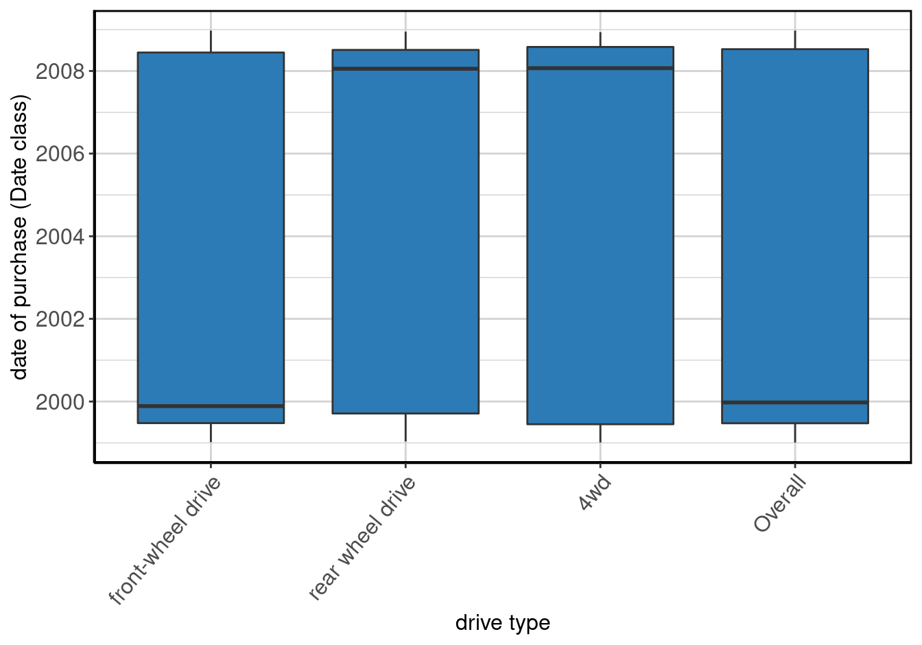
Figure 38: Boxplot of date of purchase (Date class) by drive type.
Random Numbers by Drive Type
The results are in table 58 and figure 39.
rnByDrvSummary <- data_summary(x = "rn", by = "drv", data = mpg)

make_complete_output(rnByDrvSummary)| drive type | Label | N | P NA | Mean | S Dev | Med | MAD | 25th P | 75th P | IQR | Min | Max |
|---|---|---|---|---|---|---|---|---|---|---|---|---|
| front-wheel drive | some random numbers that are generated from a normal distrubtion with mean = 10 and sd = 5 | 86 | 18.87 | 10.50 | 5.32 | 9.88 | 4.68 | 7.36 | 13.95 | 6.53 | -2.54 | 23.46 |
| rear wheel drive | some random numbers that are generated from a normal distrubtion with mean = 10 and sd = 5 | 18 | 28.00 | 11.59 | 4.49 | 11.05 | 2.89 | 9.62 | 14.28 | 4.58 | 0.28 | 20.81 |
| 4wd | some random numbers that are generated from a normal distrubtion with mean = 10 and sd = 5 | 80 | 22.33 | 10.33 | 4.99 | 11.20 | 4.60 | 6.20 | 13.08 | 6.78 | 0.57 | 23.42 |
| Overall | some random numbers that are generated from a normal distrubtion with mean = 10 and sd = 5 | 184 | 21.37 | 10.53 | 5.09 | 10.73 | 4.72 | 7.12 | 13.32 | 6.12 | -2.54 | 23.46 |
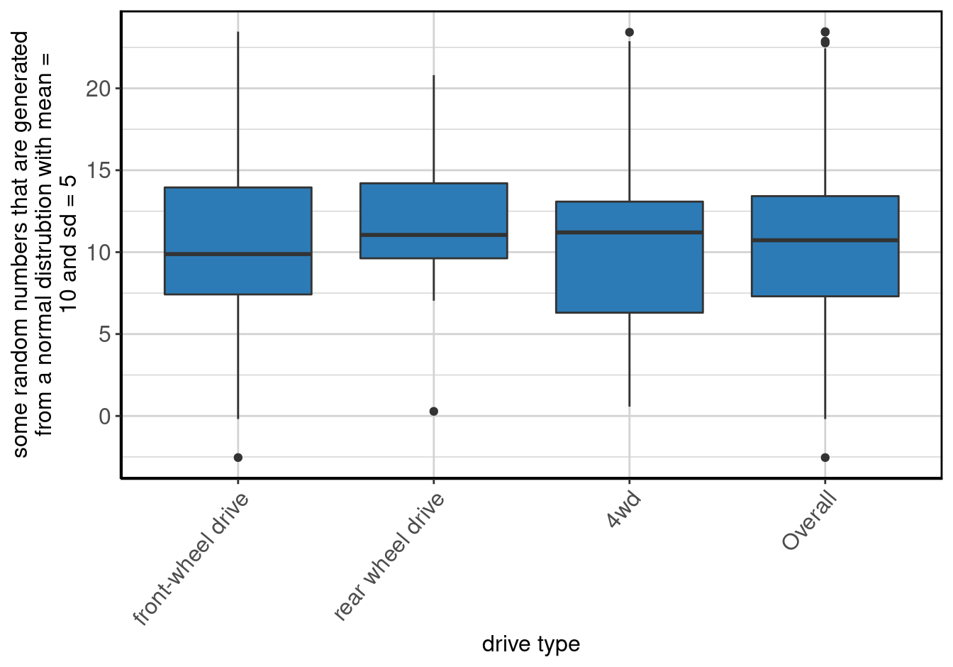
Figure 39: Boxplot of some random numbers that are generated from a normal distrubtion with mean = 10 and sd = 5 by drive type.
Random Difference in Time by Drive Type
The results are in table 59 and figure 40.
rdifftimeByDrvSummary <- data_summary(x = "rdifftime", by = "drv", difftime_units = "weeks", data = mpg)

make_complete_output(rdifftimeByDrvSummary)| drive type | Label | N | P NA | Mean | S Dev | Med | MAD | 25th P | 75th P | IQR | Min | Max |
|---|---|---|---|---|---|---|---|---|---|---|---|---|
| front-wheel drive | some random numbers that are generated from a normal distrubtion with mean = 10 and sd = 5, and then converted to weeks | 86 | 18.87 | 10.57 weeks | 5.24 weeks | 10.79 weeks | 4.80 weeks | 6.59 weeks | 13.57 weeks | 6.87 weeks | 0 weeks | 23.49 weeks |
| rear wheel drive | some random numbers that are generated from a normal distrubtion with mean = 10 and sd = 5, and then converted to weeks | 19 | 24.00 | 8.43 weeks | 5.17 weeks | 8.57 weeks | 5.74 weeks | 4.70 weeks | 12.72 weeks | 7.27 weeks | 0 weeks | 19.07 weeks |
| 4wd | some random numbers that are generated from a normal distrubtion with mean = 10 and sd = 5, and then converted to weeks | 79 | 23.30 | 9.19 weeks | 4.77 weeks | 9.02 weeks | 4.77 weeks | 6.11 weeks | 12.58 weeks | 6.15 weeks | 0 weeks | 21.71 weeks |
| Overall | some random numbers that are generated from a normal distrubtion with mean = 10 and sd = 5, and then converted to weeks | 184 | 21.37 | 9.76 weeks | 5.07 weeks | 9.60 weeks | 5.12 weeks | 6.11 weeks | 13.05 weeks | 6.79 weeks | 0 weeks | 23.49 weeks |

Figure 40: Boxplot of some random numbers that are generated from a normal distrubtion with mean = 10 and sd = 5, and then converted to weeks by drive type.
Random Difference in Time Greater than 10 by Drive Type
The results are in table 60 and figure 41.
logicalByDrvSummary <- data_summary(x = "logical", by = "drv", difftime_units = "weeks", data = mpg)

make_complete_output(logicalByDrvSummary)| some random numbers that are generated from a normal distrubtion with mean = 10 and sd = 5, and then converted to weeks, and then set to TRUE if the difference is greater than 10 | front-wheel drive | rear wheel drive | 4wd | Overall |
|---|---|---|---|---|
| FALSE | 40 (37.74%) | 11 (44%) | 45 (43.69%) | 96 (41.03%) |
| TRUE | 46 (43.4%) | 8 (32%) | 34 (33.01%) | 88 (37.61%) |
| R NA Value | 20 (18.87%) | 6 (24%) | 24 (23.3%) | 50 (21.37%) |
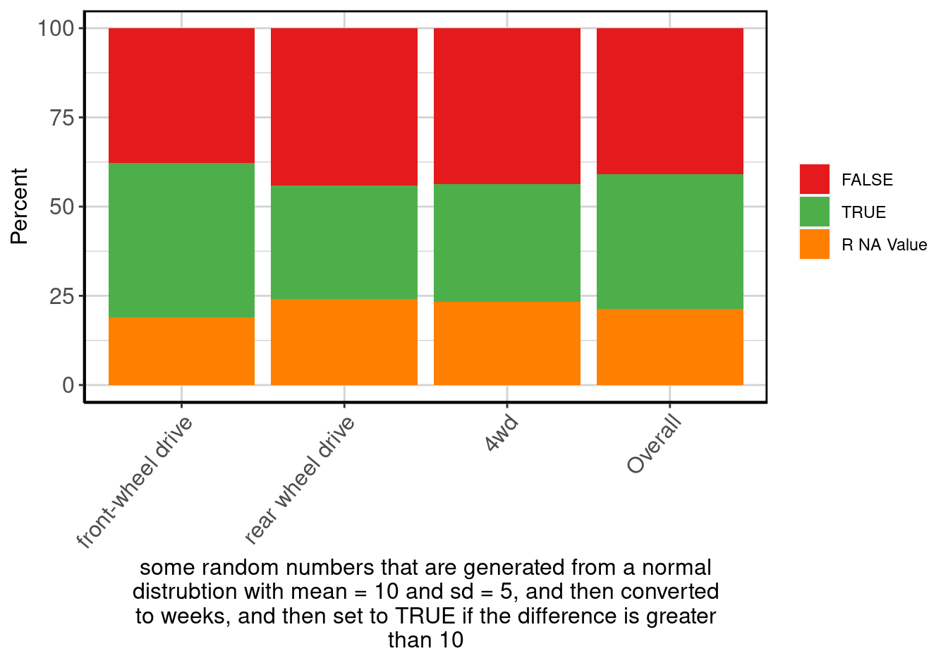
Figure 41: Stacked barplot of some random numbers that are generated from a normal distrubtion with mean = 10 and sd = 5, and then converted to weeks, and then set to TRUE if the difference is greater than 10 by drive type.
Comments by Drive Type
The results are in table 61 and figure 42.
commentsByDrvSummary <- data_summary(x = "comments", by = "drv", data = mpg)

make_complete_output(commentsByDrvSummary)| some random comments | front-wheel drive | rear wheel drive | 4wd | Overall |
|---|---|---|---|---|
| . | 9 (8.49%) | 5 (20%) | 12 (11.65%) | 26 (11.11%) |
| Blah, Blah, Blah, Blah, Blah, Blah, Blah, Blah | 12 (11.32%) | 3 (12%) | 8 (7.77%) | 23 (9.83%) |
| Does it also fly? | 11 (10.38%) | 1 (4%) | 4 (3.88%) | 16 (6.84%) |
| Does it come in green? | 12 (11.32%) | 1 (4%) | 10 (9.71%) | 23 (9.83%) |
| I like this car! | 13 (12.26%) | 1 (4%) | 10 (9.71%) | 24 (10.26%) |
| Meh. | 6 (5.66%) | 2 (8%) | 10 (9.71%) | 18 (7.69%) |
| Missing | 8 (7.55%) | 3 (12%) | 14 (13.59%) | 25 (10.68%) |
| This is the worst car ever! | 14 (13.21%) | 2 (8%) | 6 (5.83%) | 22 (9.4%) |
| want cheese flavoured cars. | 13 (12.26%) | 2 (8%) | 18 (17.48%) | 33 (14.1%) |
| R NA Value | 8 (7.55%) | 5 (20%) | 11 (10.68%) | 24 (10.26%) |
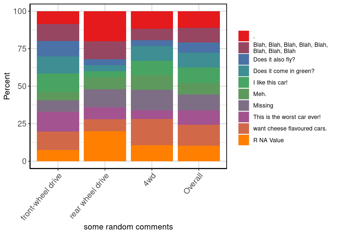
Figure 42: Stacked barplot of some random comments by drive type.
All Missing by Drive Type
The results are in table 62 and figure 43.
missByDrvSummary <- data_summary(x = "miss", by = "drv", data = mpg)

make_complete_output(missByDrvSummary)| an all missing variable | front-wheel drive | rear wheel drive | 4wd | Overall |
|---|---|---|---|---|
| R NA Value | 106 (100%) | 25 (100%) | 103 (100%) | 234 (100%) |
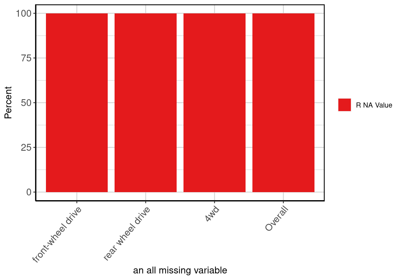
Figure 43: Stacked barplot of an all missing variable by drive type.
City and Highway MPG
City MPG by Manufacturer
The results are in table 63 and figure 44.
ctyBymanuSummary <- data_summary(x = "cty", by = "manu", data = mpg)

make_complete_output(ctyBymanuSummary)| manufacturer | Label | N | P NA | Mean | S Dev | Med | MAD | 25th P | 75th P | IQR | Min | Max |
|---|---|---|---|---|---|---|---|---|---|---|---|---|
| audi | city miles per gallon | 18 | 0 | 17.61 | 1.97 | 17.5 | 2.22 | 16 | 19 | 2.75 | 15 | 21 |
| chevrolet | city miles per gallon | 19 | 0 | 15.00 | 2.92 | 15.0 | 2.97 | 13 | 17 | 3.00 | 11 | 22 |
| dodge | city miles per gallon | 37 | 0 | 13.14 | 2.49 | 13.0 | 2.97 | 11 | 15 | 4.00 | 9 | 18 |
| ford | city miles per gallon | 25 | 0 | 14.00 | 1.91 | 14.0 | 1.48 | 13 | 15 | 2.00 | 11 | 18 |
| honda | city miles per gallon | 9 | 0 | 24.44 | 1.94 | 24.0 | 1.48 | 24 | 25 | 1.00 | 21 | 28 |
| hyundai | city miles per gallon | 14 | 0 | 18.64 | 1.50 | 18.5 | 1.48 | 18 | 20 | 1.75 | 16 | 21 |
| jeep | city miles per gallon | 8 | 0 | 13.50 | 2.51 | 14.0 | 1.48 | 11 | 15 | 2.50 | 9 | 17 |
| land rover | city miles per gallon | 4 | 0 | 11.50 | 0.58 | 11.5 | 0.74 | 11 | 12 | 1.00 | 11 | 12 |
| lincoln | city miles per gallon | 3 | 0 | 11.33 | 0.58 | 11.0 | 0.00 | 11 | 12 | 0.50 | 11 | 12 |
| mercury | city miles per gallon | 4 | 0 | 13.25 | 0.50 | 13.0 | 0.00 | 13 | 13 | 0.25 | 13 | 14 |
| nissan | city miles per gallon | 13 | 0 | 18.08 | 3.43 | 19.0 | 2.97 | 15 | 19 | 4.00 | 12 | 23 |
| pontiac | city miles per gallon | 5 | 0 | 17.00 | 1.00 | 17.0 | 1.48 | 16 | 18 | 2.00 | 16 | 18 |
| subaru | city miles per gallon | 14 | 0 | 19.29 | 0.91 | 19.0 | 1.48 | 19 | 20 | 1.00 | 18 | 21 |
| toyota | city miles per gallon | 34 | 0 | 18.53 | 4.05 | 18.0 | 4.45 | 15 | 21 | 6.00 | 11 | 28 |
| volkswagen | city miles per gallon | 27 | 0 | 20.93 | 4.56 | 21.0 | 2.97 | 18 | 21 | 2.50 | 16 | 35 |
| Overall | city miles per gallon | 234 | 0 | 16.86 | 4.26 | 17.0 | 4.45 | 14 | 19 | 5.00 | 9 | 35 |
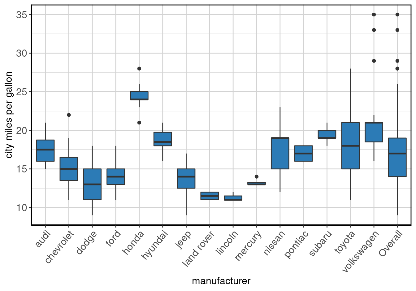
Figure 44: Boxplot of city miles per gallon by manufacturer.
Highway MPG by Manufacturer
The results are in table 64 and figure 45.
hwyBymanuSummary <- data_summary(x = "hwy", by = "manu", data = mpg)

make_complete_output(hwyBymanuSummary)| manufacturer | Label | N | P NA | Mean | S Dev | Med | MAD | 25th P | 75th P | IQR | Min | Max |
|---|---|---|---|---|---|---|---|---|---|---|---|---|
| audi | highway miles per gallon | 18 | 0 | 26.44 | 2.18 | 26.0 | 1.48 | 25 | 28 | 2.75 | 23 | 31 |
| chevrolet | highway miles per gallon | 19 | 0 | 21.89 | 5.11 | 23.0 | 5.93 | 17 | 26 | 9.00 | 14 | 30 |
| dodge | highway miles per gallon | 37 | 0 | 17.95 | 3.57 | 17.0 | 2.97 | 16 | 21 | 5.00 | 12 | 24 |
| ford | highway miles per gallon | 25 | 0 | 19.36 | 3.33 | 18.0 | 1.48 | 17 | 22 | 5.00 | 15 | 26 |
| honda | highway miles per gallon | 9 | 0 | 32.56 | 2.55 | 32.0 | 2.97 | 32 | 34 | 2.00 | 29 | 36 |
| hyundai | highway miles per gallon | 14 | 0 | 26.86 | 2.18 | 26.5 | 2.22 | 26 | 28 | 2.00 | 24 | 31 |
| jeep | highway miles per gallon | 8 | 0 | 17.62 | 3.25 | 18.5 | 2.22 | 14 | 19 | 3.00 | 12 | 22 |
| land rover | highway miles per gallon | 4 | 0 | 16.50 | 1.73 | 16.5 | 2.22 | 15 | 18 | 3.00 | 15 | 18 |
| lincoln | highway miles per gallon | 3 | 0 | 17.00 | 1.00 | 17.0 | 1.48 | 16 | 18 | 1.00 | 16 | 18 |
| mercury | highway miles per gallon | 4 | 0 | 18.00 | 1.15 | 18.0 | 1.48 | 17 | 19 | 2.00 | 17 | 19 |
| nissan | highway miles per gallon | 13 | 0 | 24.62 | 5.09 | 26.0 | 4.45 | 20 | 27 | 7.00 | 17 | 32 |
| pontiac | highway miles per gallon | 5 | 0 | 26.40 | 1.14 | 26.0 | 1.48 | 26 | 27 | 1.00 | 25 | 28 |
| subaru | highway miles per gallon | 14 | 0 | 25.57 | 1.16 | 26.0 | 1.48 | 25 | 26 | 1.00 | 23 | 27 |
| toyota | highway miles per gallon | 34 | 0 | 24.91 | 6.17 | 26.0 | 8.90 | 20 | 30 | 9.75 | 15 | 37 |
| volkswagen | highway miles per gallon | 27 | 0 | 29.22 | 5.32 | 29.0 | 1.48 | 26 | 29 | 3.00 | 23 | 44 |
| Overall | highway miles per gallon | 234 | 0 | 23.44 | 5.95 | 24.0 | 7.41 | 18 | 27 | 9.00 | 12 | 44 |
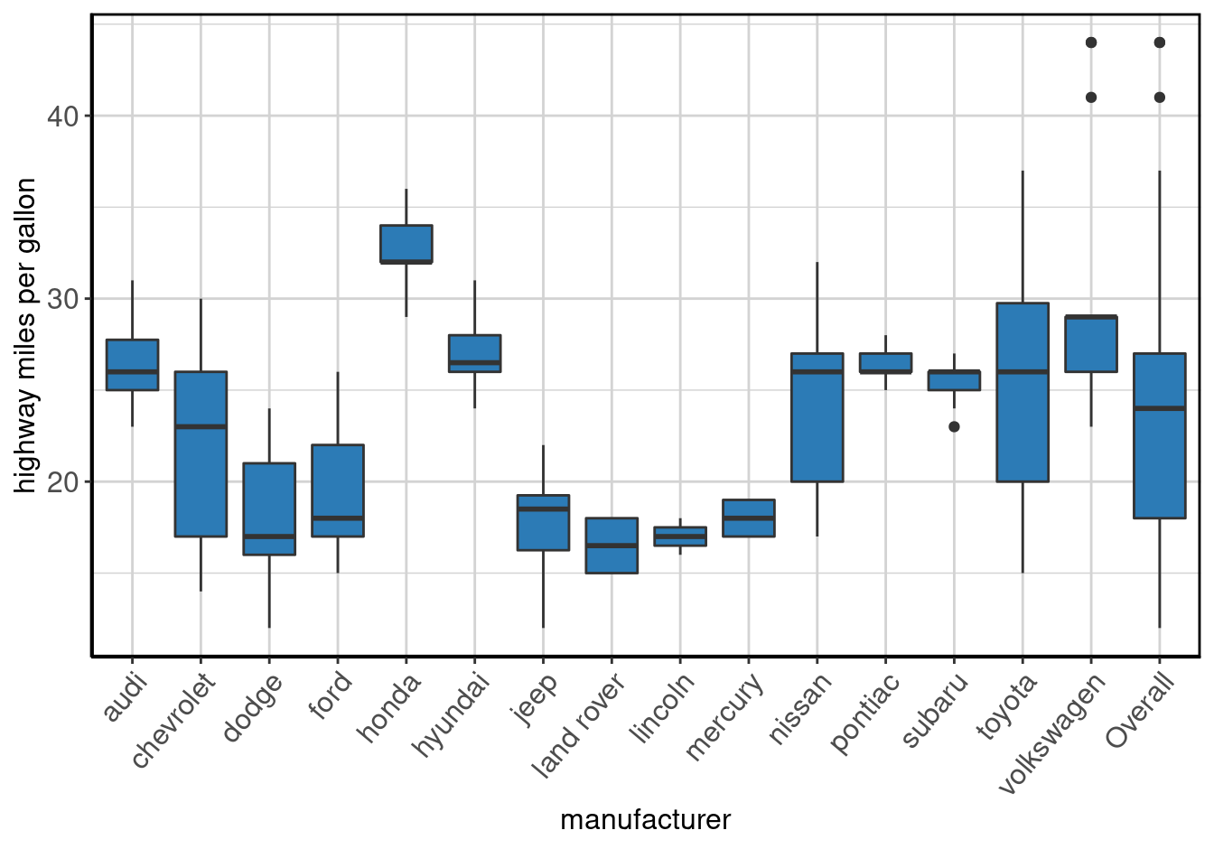
Figure 45: Boxplot of highway miles per gallon by manufacturer.
City MPG by Model Name
The results are in table 65 and figure 46.
ctyBymodelSummary <- data_summary(x = "cty", by = "model", data = mpg)

make_complete_output(ctyBymodelSummary)| model name | Label | N | P NA | Mean | S Dev | Med | MAD | 25th P | 75th P | IQR | Min | Max |
|---|---|---|---|---|---|---|---|---|---|---|---|---|
| 4runner 4wd | city miles per gallon | 6 | 0 | 15.17 | 0.75 | 15.0 | 0.74 | 15 | 16 | 0.75 | 14 | 16 |
| a4 | city miles per gallon | 7 | 0 | 18.86 | 1.86 | 18.0 | 2.97 | 18 | 21 | 2.50 | 16 | 21 |
| a4 quattro | city miles per gallon | 8 | 0 | 17.12 | 1.81 | 17.0 | 2.22 | 15 | 18 | 2.50 | 15 | 20 |
| a6 quattro | city miles per gallon | 3 | 0 | 16.00 | 1.00 | 16.0 | 1.48 | 15 | 17 | 1.00 | 15 | 17 |
| altima | city miles per gallon | 6 | 0 | 20.67 | 1.97 | 20.0 | 1.48 | 19 | 23 | 3.50 | 19 | 23 |
| c1500 suburban 2wd | city miles per gallon | 5 | 0 | 12.80 | 1.30 | 13.0 | 1.48 | 12 | 14 | 2.00 | 11 | 14 |
| camry | city miles per gallon | 7 | 0 | 19.86 | 1.46 | 21.0 | 0.00 | 18 | 21 | 2.50 | 18 | 21 |
| camry solara | city miles per gallon | 7 | 0 | 19.86 | 1.77 | 21.0 | 1.48 | 18 | 21 | 3.00 | 18 | 22 |
| caravan 2wd | city miles per gallon | 11 | 0 | 15.82 | 1.83 | 16.0 | 1.48 | 15 | 17 | 1.50 | 11 | 18 |
| civic | city miles per gallon | 9 | 0 | 24.44 | 1.94 | 24.0 | 1.48 | 24 | 25 | 1.00 | 21 | 28 |
| corolla | city miles per gallon | 5 | 0 | 25.60 | 1.67 | 26.0 | 2.97 | 24 | 26 | 2.00 | 24 | 28 |
| corvette | city miles per gallon | 5 | 0 | 15.40 | 0.55 | 15.0 | 0.00 | 15 | 16 | 1.00 | 15 | 16 |
| dakota pickup 4wd | city miles per gallon | 9 | 0 | 12.78 | 1.99 | 14.0 | 1.48 | 11 | 14 | 3.00 | 9 | 15 |
| durango 4wd | city miles per gallon | 7 | 0 | 11.86 | 1.57 | 13.0 | 0.00 | 11 | 13 | 2.00 | 9 | 13 |
| expedition 2wd | city miles per gallon | 3 | 0 | 11.33 | 0.58 | 11.0 | 0.00 | 11 | 12 | 0.50 | 11 | 12 |
| explorer 4wd | city miles per gallon | 6 | 0 | 13.67 | 0.82 | 13.5 | 0.74 | 13 | 14 | 1.00 | 13 | 15 |
| f150 pickup 4wd | city miles per gallon | 7 | 0 | 13.00 | 1.00 | 13.0 | 0.00 | 13 | 14 | 0.50 | 11 | 14 |
| forester awd | city miles per gallon | 6 | 0 | 18.83 | 0.98 | 18.5 | 0.74 | 18 | 20 | 1.75 | 18 | 20 |
| grand cherokee 4wd | city miles per gallon | 8 | 0 | 13.50 | 2.51 | 14.0 | 1.48 | 11 | 15 | 2.50 | 9 | 17 |
| grand prix | city miles per gallon | 5 | 0 | 17.00 | 1.00 | 17.0 | 1.48 | 16 | 18 | 2.00 | 16 | 18 |
| gti | city miles per gallon | 5 | 0 | 20.00 | 2.00 | 21.0 | 1.48 | 19 | 21 | 2.00 | 17 | 22 |
| impreza awd | city miles per gallon | 8 | 0 | 19.62 | 0.74 | 19.5 | 0.74 | 19 | 20 | 1.00 | 19 | 21 |
| jetta | city miles per gallon | 9 | 0 | 21.22 | 4.87 | 21.0 | 1.48 | 19 | 21 | 2.00 | 16 | 33 |
| k1500 tahoe 4wd | city miles per gallon | 4 | 0 | 12.50 | 1.73 | 12.5 | 2.22 | 11 | 14 | 3.00 | 11 | 14 |
| land cruiser wagon 4wd | city miles per gallon | 2 | 0 | 12.00 | 1.41 | 12.0 | 1.48 | 11 | 13 | 1.00 | 11 | 13 |
| malibu | city miles per gallon | 5 | 0 | 18.80 | 1.92 | 18.0 | 1.48 | 18 | 19 | 1.00 | 17 | 22 |
| maxima | city miles per gallon | 3 | 0 | 18.67 | 0.58 | 19.0 | 0.00 | 18 | 19 | 0.50 | 18 | 19 |
| mountaineer 4wd | city miles per gallon | 4 | 0 | 13.25 | 0.50 | 13.0 | 0.00 | 13 | 13 | 0.25 | 13 | 14 |
| mustang | city miles per gallon | 9 | 0 | 15.89 | 1.45 | 15.0 | 1.48 | 15 | 17 | 2.00 | 14 | 18 |
| navigator 2wd | city miles per gallon | 3 | 0 | 11.33 | 0.58 | 11.0 | 0.00 | 11 | 12 | 0.50 | 11 | 12 |
| new beetle | city miles per gallon | 6 | 0 | 24.00 | 6.51 | 20.5 | 1.48 | 20 | 29 | 7.00 | 19 | 35 |
| passat | city miles per gallon | 7 | 0 | 18.57 | 1.90 | 18.0 | 1.48 | 17 | 21 | 2.50 | 16 | 21 |
| pathfinder 4wd | city miles per gallon | 4 | 0 | 13.75 | 1.26 | 14.0 | 0.74 | 12 | 14 | 0.75 | 12 | 15 |
| ram 1500 pickup 4wd | city miles per gallon | 10 | 0 | 11.40 | 1.51 | 11.5 | 1.48 | 11 | 13 | 1.75 | 9 | 13 |
| range rover | city miles per gallon | 4 | 0 | 11.50 | 0.58 | 11.5 | 0.74 | 11 | 12 | 1.00 | 11 | 12 |
| sonata | city miles per gallon | 7 | 0 | 19.00 | 1.41 | 18.0 | 0.00 | 18 | 21 | 2.00 | 18 | 21 |
| tiburon | city miles per gallon | 7 | 0 | 18.29 | 1.60 | 19.0 | 1.48 | 17 | 20 | 2.50 | 16 | 20 |
| toyota tacoma 4wd | city miles per gallon | 7 | 0 | 15.57 | 0.79 | 15.0 | 0.00 | 15 | 16 | 1.00 | 15 | 17 |
| Overall | city miles per gallon | 234 | 0 | 16.86 | 4.26 | 17.0 | 4.45 | 14 | 19 | 5.00 | 9 | 35 |
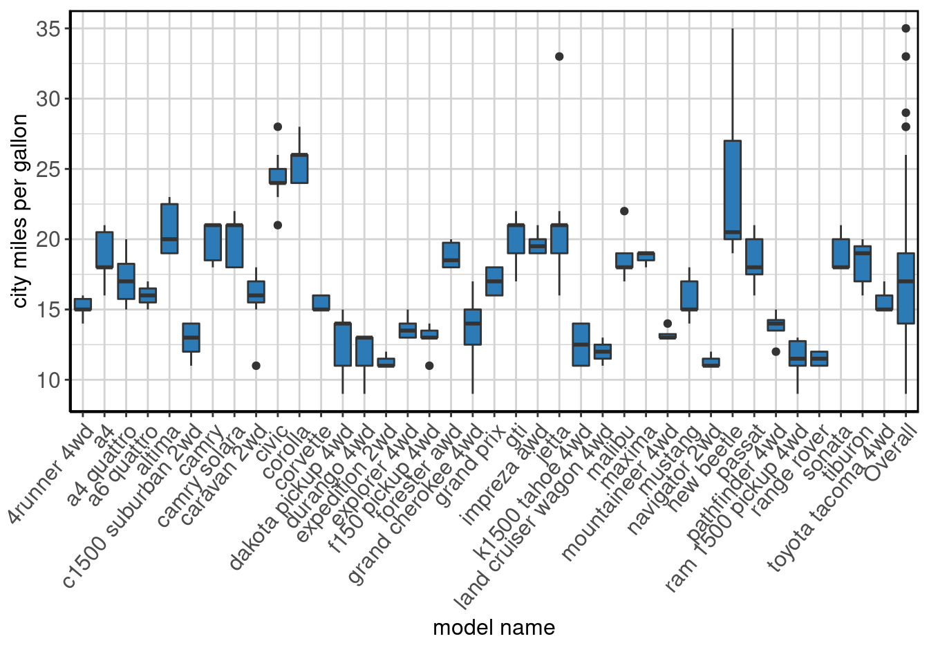
Figure 46: Boxplot of city miles per gallon by model name.
Highway MPG by Model Name
The results are in table 66 and figure 47.
hwyBymodelSummary <- data_summary(x = "hwy", by = "model", data = mpg)

make_complete_output(hwyBymodelSummary)| model name | Label | N | P NA | Mean | S Dev | Med | MAD | 25th P | 75th P | IQR | Min | Max |
|---|---|---|---|---|---|---|---|---|---|---|---|---|
| 4runner 4wd | highway miles per gallon | 6 | 0 | 18.83 | 1.47 | 19.5 | 0.74 | 17 | 20 | 2.50 | 17 | 20 |
| a4 | highway miles per gallon | 7 | 0 | 28.29 | 1.98 | 29.0 | 2.97 | 26 | 30 | 3.00 | 26 | 31 |
| a4 quattro | highway miles per gallon | 8 | 0 | 25.75 | 1.16 | 25.0 | 0.00 | 25 | 26 | 1.25 | 25 | 28 |
| a6 quattro | highway miles per gallon | 3 | 0 | 24.00 | 1.00 | 24.0 | 1.48 | 23 | 25 | 1.00 | 23 | 25 |
| altima | highway miles per gallon | 6 | 0 | 28.67 | 2.42 | 28.0 | 2.22 | 27 | 31 | 3.50 | 26 | 32 |
| c1500 suburban 2wd | highway miles per gallon | 5 | 0 | 17.80 | 2.17 | 17.0 | 2.97 | 17 | 20 | 3.00 | 15 | 20 |
| camry | highway miles per gallon | 7 | 0 | 28.29 | 2.14 | 28.0 | 2.97 | 26 | 31 | 3.50 | 26 | 31 |
| camry solara | highway miles per gallon | 7 | 0 | 28.14 | 2.19 | 27.0 | 1.48 | 26 | 31 | 3.50 | 26 | 31 |
| caravan 2wd | highway miles per gallon | 11 | 0 | 22.36 | 2.06 | 23.0 | 1.48 | 22 | 24 | 2.00 | 17 | 24 |
| civic | highway miles per gallon | 9 | 0 | 32.56 | 2.55 | 32.0 | 2.97 | 32 | 34 | 2.00 | 29 | 36 |
| corolla | highway miles per gallon | 5 | 0 | 34.00 | 2.65 | 35.0 | 2.97 | 33 | 35 | 2.00 | 30 | 37 |
| corvette | highway miles per gallon | 5 | 0 | 24.80 | 1.30 | 25.0 | 1.48 | 24 | 26 | 2.00 | 23 | 26 |
| dakota pickup 4wd | highway miles per gallon | 9 | 0 | 17.00 | 2.29 | 17.0 | 2.97 | 17 | 19 | 2.00 | 12 | 19 |
| durango 4wd | highway miles per gallon | 7 | 0 | 16.00 | 2.00 | 17.0 | 1.48 | 15 | 17 | 1.50 | 12 | 18 |
| expedition 2wd | highway miles per gallon | 3 | 0 | 17.33 | 0.58 | 17.0 | 0.00 | 17 | 18 | 0.50 | 17 | 18 |
| explorer 4wd | highway miles per gallon | 6 | 0 | 18.00 | 1.10 | 18.0 | 1.48 | 17 | 19 | 2.00 | 17 | 19 |
| f150 pickup 4wd | highway miles per gallon | 7 | 0 | 16.43 | 0.79 | 17.0 | 0.00 | 16 | 17 | 1.00 | 15 | 17 |
| forester awd | highway miles per gallon | 6 | 0 | 25.00 | 1.41 | 25.0 | 1.48 | 24 | 26 | 1.50 | 23 | 27 |
| grand cherokee 4wd | highway miles per gallon | 8 | 0 | 17.62 | 3.25 | 18.5 | 2.22 | 14 | 19 | 3.00 | 12 | 22 |
| grand prix | highway miles per gallon | 5 | 0 | 26.40 | 1.14 | 26.0 | 1.48 | 26 | 27 | 1.00 | 25 | 28 |
| gti | highway miles per gallon | 5 | 0 | 27.40 | 2.30 | 29.0 | 0.00 | 26 | 29 | 3.00 | 24 | 29 |
| impreza awd | highway miles per gallon | 8 | 0 | 26.00 | 0.76 | 26.0 | 0.74 | 25 | 26 | 0.50 | 25 | 27 |
| jetta | highway miles per gallon | 9 | 0 | 29.11 | 6.07 | 29.0 | 0.00 | 26 | 29 | 3.00 | 23 | 44 |
| k1500 tahoe 4wd | highway miles per gallon | 4 | 0 | 16.25 | 2.22 | 16.0 | 2.22 | 14 | 17 | 2.75 | 14 | 19 |
| land cruiser wagon 4wd | highway miles per gallon | 2 | 0 | 16.50 | 2.12 | 16.5 | 2.22 | 15 | 18 | 1.50 | 15 | 18 |
| malibu | highway miles per gallon | 5 | 0 | 27.60 | 1.82 | 27.0 | 1.48 | 26 | 29 | 3.00 | 26 | 30 |
| maxima | highway miles per gallon | 3 | 0 | 25.33 | 0.58 | 25.0 | 0.00 | 25 | 26 | 0.50 | 25 | 26 |
| mountaineer 4wd | highway miles per gallon | 4 | 0 | 18.00 | 1.15 | 18.0 | 1.48 | 17 | 19 | 2.00 | 17 | 19 |
| mustang | highway miles per gallon | 9 | 0 | 23.22 | 2.17 | 23.0 | 2.97 | 22 | 25 | 3.00 | 20 | 26 |
| navigator 2wd | highway miles per gallon | 3 | 0 | 17.00 | 1.00 | 17.0 | 1.48 | 16 | 18 | 1.00 | 16 | 18 |
| new beetle | highway miles per gallon | 6 | 0 | 32.83 | 7.63 | 29.0 | 2.97 | 28 | 41 | 9.75 | 26 | 44 |
| passat | highway miles per gallon | 7 | 0 | 27.57 | 1.51 | 28.0 | 1.48 | 26 | 29 | 3.00 | 26 | 29 |
| pathfinder 4wd | highway miles per gallon | 4 | 0 | 18.00 | 1.41 | 17.5 | 0.74 | 17 | 18 | 1.50 | 17 | 20 |
| ram 1500 pickup 4wd | highway miles per gallon | 10 | 0 | 15.30 | 1.89 | 16.0 | 1.48 | 15 | 17 | 1.75 | 12 | 17 |
| range rover | highway miles per gallon | 4 | 0 | 16.50 | 1.73 | 16.5 | 2.22 | 15 | 18 | 3.00 | 15 | 18 |
| sonata | highway miles per gallon | 7 | 0 | 27.71 | 2.06 | 27.0 | 1.48 | 26 | 30 | 3.00 | 26 | 31 |
| tiburon | highway miles per gallon | 7 | 0 | 26.00 | 2.08 | 26.0 | 2.97 | 24 | 28 | 3.50 | 24 | 29 |
| toyota tacoma 4wd | highway miles per gallon | 7 | 0 | 19.43 | 1.62 | 20.0 | 1.48 | 18 | 20 | 1.50 | 17 | 22 |
| Overall | highway miles per gallon | 234 | 0 | 23.44 | 5.95 | 24.0 | 7.41 | 18 | 27 | 9.00 | 12 | 44 |
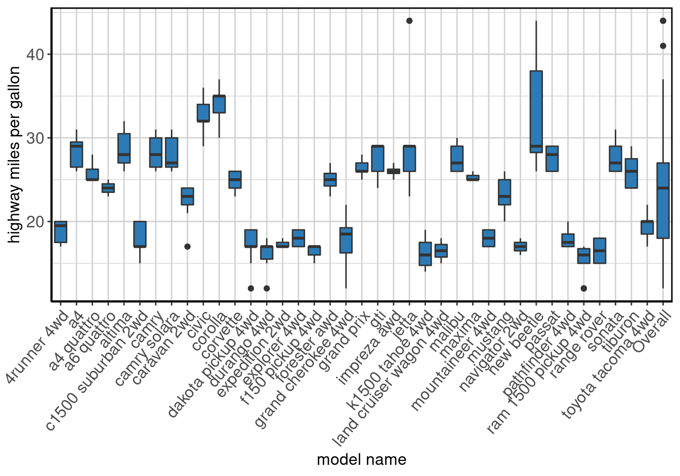
Figure 47: Boxplot of highway miles per gallon by model name.
City MPG by Year of Manufacture
The results are in table 67 and figure 48.
ctyByYearSummary <- data_summary(x = "cty", by = "year", data = mpg)

make_complete_output(ctyByYearSummary)| year of manufacture | Label | N | P NA | Mean | S Dev | Med | MAD | 25th P | 75th P | IQR | Min | Max |
|---|---|---|---|---|---|---|---|---|---|---|---|---|
| 1999 | city miles per gallon | 117 | 0 | 17.02 | 4.46 | 17 | 2.97 | 14 | 19 | 5 | 11 | 35 |
| 2008 | city miles per gallon | 117 | 0 | 16.70 | 4.06 | 17 | 4.45 | 13 | 20 | 7 | 9 | 28 |
| Overall | city miles per gallon | 234 | 0 | 16.86 | 4.26 | 17 | 4.45 | 14 | 19 | 5 | 9 | 35 |
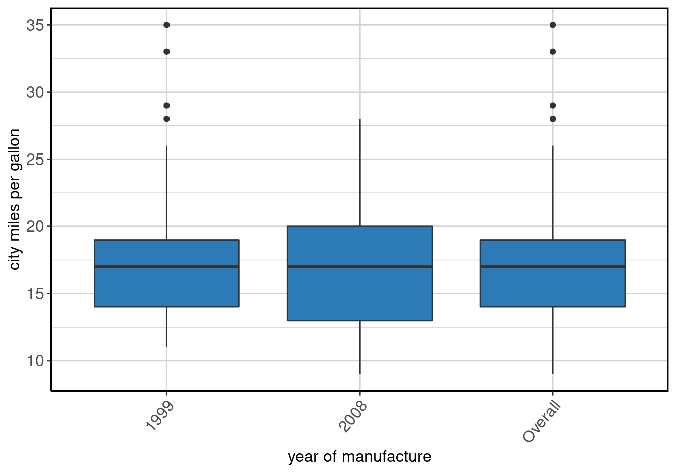
Figure 48: Boxplot of city miles per gallon by year of manufacture.
Highway MPG by Year of Manufacture
The results are in table 68 and figure 49.
hwyByYearSummary <- data_summary(x = "hwy", by = "year", data = mpg)

make_complete_output(hwyByYearSummary)| year of manufacture | Label | N | P NA | Mean | S Dev | Med | MAD | 25th P | 75th P | IQR | Min | Max |
|---|---|---|---|---|---|---|---|---|---|---|---|---|
| 1999 | highway miles per gallon | 117 | 0 | 23.43 | 6.08 | 25 | 5.93 | 17 | 26 | 9 | 15 | 44 |
| 2008 | highway miles per gallon | 117 | 0 | 23.45 | 5.85 | 24 | 7.41 | 18 | 28 | 10 | 12 | 37 |
| Overall | highway miles per gallon | 234 | 0 | 23.44 | 5.95 | 24 | 7.41 | 18 | 27 | 9 | 12 | 44 |
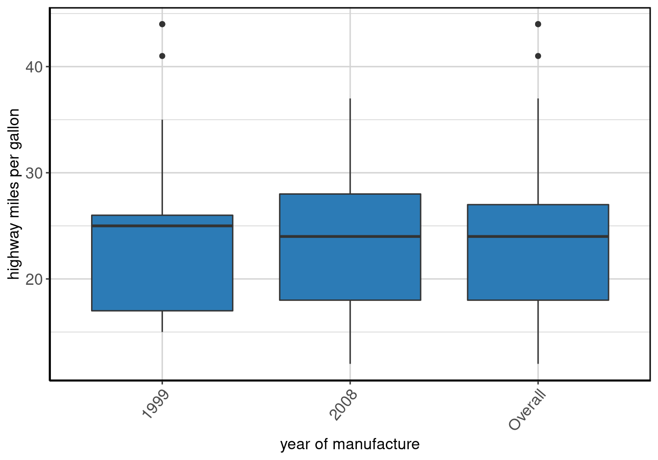
Figure 49: Boxplot of highway miles per gallon by year of manufacture.
City MPG by Number of Cylinders
The results are in table 69 and figure 50.
ctyByCylSummary <- data_summary(x = "cty", by = "cyl", data = mpg)

make_complete_output(ctyByCylSummary)| number of cylinders | Label | N | P NA | Mean | S Dev | Med | MAD | 25th P | 75th P | IQR | Min | Max |
|---|---|---|---|---|---|---|---|---|---|---|---|---|
| 4 | city miles per gallon | 81 | 0 | 21.01 | 3.50 | 21.0 | 2.97 | 19 | 22 | 3 | 15 | 35 |
| 5 | city miles per gallon | 4 | 0 | 20.50 | 0.58 | 20.5 | 0.74 | 20 | 21 | 1 | 20 | 21 |
| 6 | city miles per gallon | 79 | 0 | 16.22 | 1.77 | 16.0 | 1.48 | 15 | 18 | 3 | 11 | 19 |
| 8 | city miles per gallon | 70 | 0 | 12.57 | 1.81 | 13.0 | 2.22 | 11 | 14 | 3 | 9 | 16 |
| Overall | city miles per gallon | 234 | 0 | 16.86 | 4.26 | 17.0 | 4.45 | 14 | 19 | 5 | 9 | 35 |

Figure 50: Boxplot of city miles per gallon by number of cylinders.
Highway MPG by Number of Cylinders
The results are in table 70 and figure 51.
hwyByCylSummary <- data_summary(x = "hwy", by = "cyl", data = mpg)

make_complete_output(hwyByCylSummary)| number of cylinders | Label | N | P NA | Mean | S Dev | Med | MAD | 25th P | 75th P | IQR | Min | Max |
|---|---|---|---|---|---|---|---|---|---|---|---|---|
| 4 | highway miles per gallon | 81 | 0 | 28.80 | 4.52 | 29 | 2.97 | 26 | 31 | 5.00 | 20 | 44 |
| 5 | highway miles per gallon | 4 | 0 | 28.75 | 0.50 | 29 | 0.00 | 28 | 29 | 0.25 | 28 | 29 |
| 6 | highway miles per gallon | 79 | 0 | 22.82 | 3.69 | 24 | 2.97 | 19 | 26 | 7.00 | 17 | 29 |
| 8 | highway miles per gallon | 70 | 0 | 17.63 | 3.26 | 17 | 2.97 | 16 | 19 | 3.00 | 12 | 26 |
| Overall | highway miles per gallon | 234 | 0 | 23.44 | 5.95 | 24 | 7.41 | 18 | 27 | 9.00 | 12 | 44 |
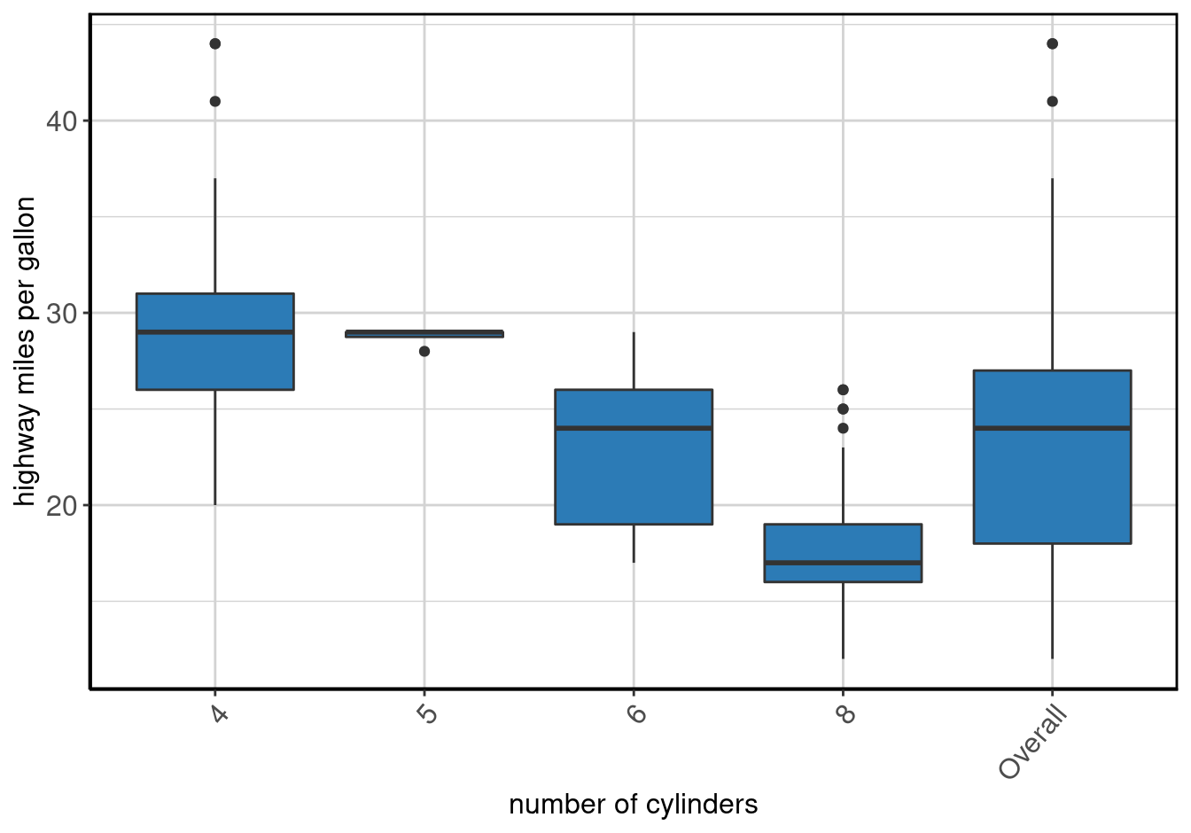
Figure 51: Boxplot of highway miles per gallon by number of cylinders.
City MPG by Type of Transmission
The results are in table 71 and figure 52.
ctyBytransSummary <- data_summary(x = "cty", by = "trans", data = mpg)

make_complete_output(ctyBytransSummary)| type of transmission | Label | N | P NA | Mean | S Dev | Med | MAD | 25th P | 75th P | IQR | Min | Max |
|---|---|---|---|---|---|---|---|---|---|---|---|---|
| auto(av) | city miles per gallon | 5 | 0 | 20.00 | 2.00 | 19 | 1.48 | 19 | 21 | 2.0 | 18 | 23 |
| auto(l3) | city miles per gallon | 2 | 0 | 21.00 | 4.24 | 21 | 4.45 | 18 | 24 | 3.0 | 18 | 24 |
| auto(l4) | city miles per gallon | 83 | 0 | 15.94 | 3.98 | 16 | 4.45 | 13 | 18 | 5.0 | 11 | 29 |
| auto(l5) | city miles per gallon | 39 | 0 | 14.72 | 3.49 | 14 | 1.48 | 13 | 16 | 3.0 | 9 | 25 |
| auto(l6) | city miles per gallon | 6 | 0 | 13.67 | 1.86 | 13 | 1.48 | 12 | 16 | 3.0 | 12 | 16 |
| auto(s4) | city miles per gallon | 3 | 0 | 18.67 | 2.31 | 20 | 0.00 | 16 | 20 | 2.0 | 16 | 20 |
| auto(s5) | city miles per gallon | 3 | 0 | 17.33 | 5.03 | 18 | 5.93 | 12 | 22 | 5.0 | 12 | 22 |
| auto(s6) | city miles per gallon | 16 | 0 | 17.38 | 3.22 | 17 | 2.97 | 15 | 19 | 3.5 | 12 | 22 |
| manual(m5) | city miles per gallon | 58 | 0 | 19.26 | 4.56 | 19 | 2.97 | 17 | 21 | 4.0 | 11 | 35 |
| manual(m6) | city miles per gallon | 19 | 0 | 16.89 | 3.83 | 16 | 5.93 | 15 | 21 | 5.5 | 9 | 23 |
| Overall | city miles per gallon | 234 | 0 | 16.86 | 4.26 | 17 | 4.45 | 14 | 19 | 5.0 | 9 | 35 |
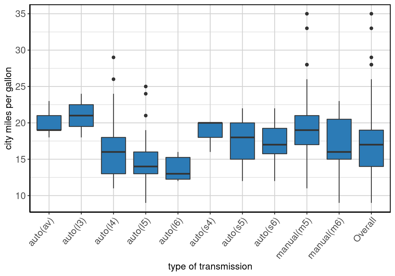
Figure 52: Boxplot of city miles per gallon by type of transmission.
Highway MPG by Type of Transmission
The results are in table 72 and figure 53.
hwyBytransSummary <- data_summary(x = "hwy", by = "trans", data = mpg)

make_complete_output(hwyBytransSummary)| type of transmission | Label | N | P NA | Mean | S Dev | Med | MAD | 25th P | 75th P | IQR | Min | Max |
|---|---|---|---|---|---|---|---|---|---|---|---|---|
| auto(av) | highway miles per gallon | 5 | 0 | 27.80 | 2.59 | 27 | 2.97 | 26 | 30 | 4.00 | 25 | 31 |
| auto(l3) | highway miles per gallon | 2 | 0 | 27.00 | 4.24 | 27 | 4.45 | 24 | 30 | 3.00 | 24 | 30 |
| auto(l4) | highway miles per gallon | 83 | 0 | 21.96 | 5.64 | 22 | 7.41 | 17 | 26 | 9.00 | 14 | 41 |
| auto(l5) | highway miles per gallon | 39 | 0 | 20.72 | 6.04 | 19 | 2.97 | 17 | 25 | 7.50 | 12 | 36 |
| auto(l6) | highway miles per gallon | 6 | 0 | 20.00 | 2.37 | 19 | 1.48 | 18 | 23 | 3.75 | 18 | 23 |
| auto(s4) | highway miles per gallon | 3 | 0 | 25.67 | 1.15 | 25 | 0.00 | 25 | 27 | 1.00 | 25 | 27 |
| auto(s5) | highway miles per gallon | 3 | 0 | 25.33 | 6.66 | 27 | 5.93 | 18 | 31 | 6.50 | 18 | 31 |
| auto(s6) | highway miles per gallon | 16 | 0 | 25.19 | 3.99 | 26 | 3.71 | 23 | 28 | 3.75 | 18 | 29 |
| manual(m5) | highway miles per gallon | 58 | 0 | 26.29 | 5.99 | 26 | 4.45 | 24 | 29 | 5.00 | 16 | 44 |
| manual(m6) | highway miles per gallon | 19 | 0 | 24.21 | 5.75 | 26 | 4.45 | 19 | 29 | 9.50 | 12 | 32 |
| Overall | highway miles per gallon | 234 | 0 | 23.44 | 5.95 | 24 | 7.41 | 18 | 27 | 9.00 | 12 | 44 |
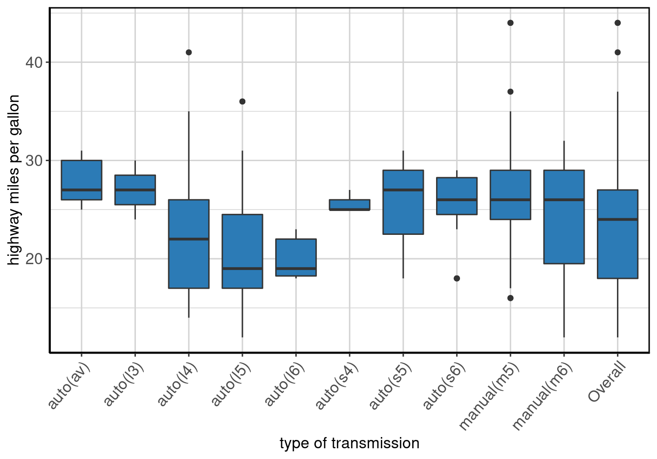
Figure 53: Boxplot of highway miles per gallon by type of transmission.
City MPG by Drive Type
The results are in table 73 and figure 54.
ctyByDrvSummary <- data_summary(x = "cty", by = "drv", data = mpg)

make_complete_output(ctyByDrvSummary)| drive type | Label | N | P NA | Mean | S Dev | Med | MAD | 25th P | 75th P | IQR | Min | Max |
|---|---|---|---|---|---|---|---|---|---|---|---|---|
| front-wheel drive | city miles per gallon | 106 | 0 | 19.97 | 3.63 | 19 | 2.97 | 18 | 21 | 3 | 11 | 35 |
| rear wheel drive | city miles per gallon | 25 | 0 | 14.08 | 2.22 | 15 | 1.48 | 12 | 15 | 3 | 11 | 18 |
| 4wd | city miles per gallon | 103 | 0 | 14.33 | 2.87 | 14 | 2.97 | 13 | 16 | 3 | 9 | 21 |
| Overall | city miles per gallon | 234 | 0 | 16.86 | 4.26 | 17 | 4.45 | 14 | 19 | 5 | 9 | 35 |
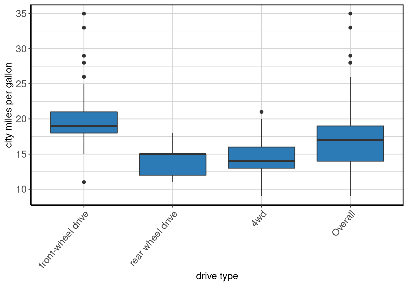
Figure 54: Boxplot of city miles per gallon by drive type.
Highway MPG by Drive Type
The results are in table 74 and figure 55.
hwyByDrvSummary <- data_summary(x = "hwy", by = "drv", data = mpg)

make_complete_output(hwyByDrvSummary)| drive type | Label | N | P NA | Mean | S Dev | Med | MAD | 25th P | 75th P | IQR | Min | Max |
|---|---|---|---|---|---|---|---|---|---|---|---|---|
| front-wheel drive | highway miles per gallon | 106 | 0 | 28.16 | 4.21 | 28 | 2.97 | 26 | 29 | 3 | 17 | 44 |
| rear wheel drive | highway miles per gallon | 25 | 0 | 21.00 | 3.66 | 21 | 5.93 | 17 | 24 | 7 | 15 | 26 |
| 4wd | highway miles per gallon | 103 | 0 | 19.17 | 4.08 | 18 | 2.97 | 17 | 22 | 5 | 12 | 28 |
| Overall | highway miles per gallon | 234 | 0 | 23.44 | 5.95 | 24 | 7.41 | 18 | 27 | 9 | 12 | 44 |
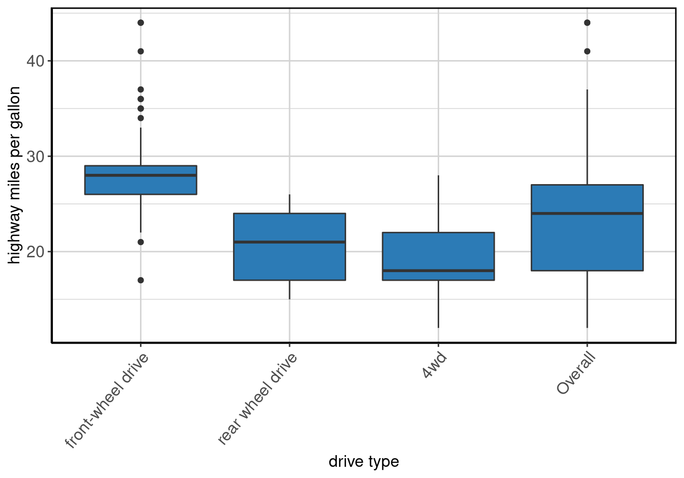
Figure 55: Boxplot of highway miles per gallon by drive type.
City MPG by Fuel Type
The results are in table 75 and figure 56.
ctyByflSummary <- data_summary(x = "cty", by = "fl", data = mpg)

make_complete_output(ctyByflSummary)| fuel type | Label | N | P NA | Mean | S Dev | Med | MAD | 25th P | 75th P | IQR | Min | Max |
|---|---|---|---|---|---|---|---|---|---|---|---|---|
| c | city miles per gallon | 1 | 0 | 24.00 | NA | 24 | 0.00 | 24 | 24 | 0.0 | 24 | 24 |
| d | city miles per gallon | 5 | 0 | 25.60 | 9.53 | 29 | 8.90 | 17 | 33 | 16.0 | 14 | 35 |
| e | city miles per gallon | 8 | 0 | 9.75 | 1.04 | 9 | 0.00 | 9 | 11 | 2.0 | 9 | 11 |
| p | city miles per gallon | 52 | 0 | 17.37 | 3.04 | 18 | 2.97 | 15 | 19 | 3.5 | 11 | 23 |
| r | city miles per gallon | 168 | 0 | 16.74 | 3.89 | 16 | 4.45 | 14 | 19 | 5.0 | 11 | 28 |
| Overall | city miles per gallon | 234 | 0 | 16.86 | 4.26 | 17 | 4.45 | 14 | 19 | 5.0 | 9 | 35 |
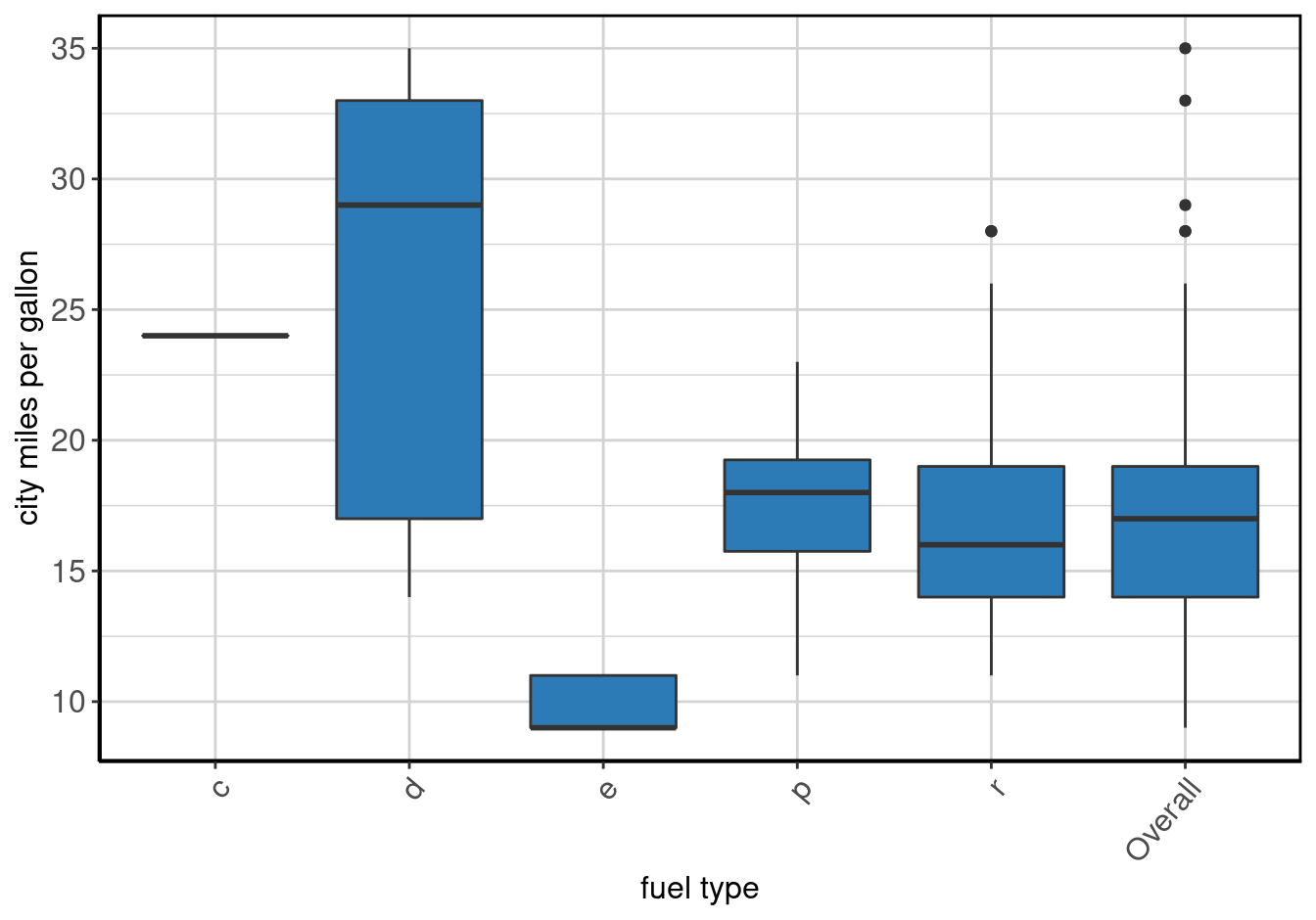
Figure 56: Boxplot of city miles per gallon by fuel type.
Highway MPG by Fuel Type
The results are in table 76 and figure 57.
hwyByflSummary <- data_summary(x = "hwy", by = "fl", data = mpg)

make_complete_output(hwyByflSummary)| fuel type | Label | N | P NA | Mean | S Dev | Med | MAD | 25th P | 75th P | IQR | Min | Max |
|---|---|---|---|---|---|---|---|---|---|---|---|---|
| c | highway miles per gallon | 1 | 0 | 36.00 | NA | 36 | 0.00 | 36 | 36 | 0.00 | 36 | 36 |
| d | highway miles per gallon | 5 | 0 | 33.60 | 13.05 | 41 | 4.45 | 22 | 44 | 22.00 | 17 | 44 |
| e | highway miles per gallon | 8 | 0 | 13.25 | 1.91 | 12 | 0.00 | 12 | 14 | 2.25 | 12 | 17 |
| p | highway miles per gallon | 52 | 0 | 25.23 | 3.93 | 26 | 2.97 | 25 | 28 | 3.25 | 14 | 31 |
| r | highway miles per gallon | 168 | 0 | 22.99 | 5.51 | 23 | 7.41 | 17 | 27 | 9.25 | 15 | 37 |
| Overall | highway miles per gallon | 234 | 0 | 23.44 | 5.95 | 24 | 7.41 | 18 | 27 | 9.00 | 12 | 44 |
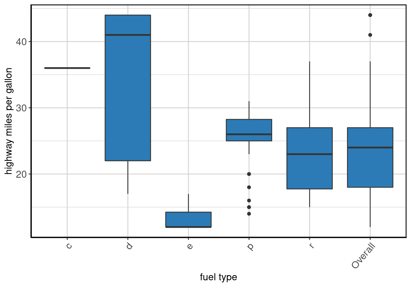
Figure 57: Boxplot of highway miles per gallon by fuel type.
City MPG by Type of Car
The results are in table 77 and figure 58.
ctyByclassSummary <- data_summary(x = "cty", by = "class", data = mpg)

make_complete_output(ctyByclassSummary)| type of car | Label | N | P NA | Mean | S Dev | Med | MAD | 25th P | 75th P | IQR | Min | Max |
|---|---|---|---|---|---|---|---|---|---|---|---|---|
| 2seater | city miles per gallon | 5 | 0 | 15.40 | 0.55 | 15 | 0.00 | 15 | 16 | 1.00 | 15 | 16 |
| compact | city miles per gallon | 47 | 0 | 20.13 | 3.39 | 20 | 2.97 | 18 | 21 | 3.00 | 15 | 33 |
| midsize | city miles per gallon | 41 | 0 | 18.76 | 1.95 | 18 | 1.48 | 18 | 21 | 3.00 | 15 | 23 |
| minivan | city miles per gallon | 11 | 0 | 15.82 | 1.83 | 16 | 1.48 | 15 | 17 | 1.50 | 11 | 18 |
| pickup | city miles per gallon | 33 | 0 | 13.00 | 2.05 | 13 | 2.97 | 11 | 14 | 3.00 | 9 | 17 |
| subcompact | city miles per gallon | 35 | 0 | 20.37 | 4.60 | 19 | 2.97 | 17 | 24 | 6.50 | 14 | 35 |
| suv | city miles per gallon | 62 | 0 | 13.50 | 2.42 | 13 | 2.22 | 12 | 15 | 2.75 | 9 | 20 |
| Overall | city miles per gallon | 234 | 0 | 16.86 | 4.26 | 17 | 4.45 | 14 | 19 | 5.00 | 9 | 35 |
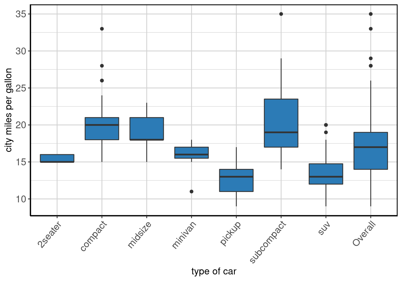
Figure 58: Boxplot of city miles per gallon by type of car.
Highway MPG by Type of Car
The results are in table 78 and figure 59.
hwyByclassSummary <- data_summary(x = "hwy", by = "class", data = mpg)

make_complete_output(hwyByclassSummary)| type of car | Label | N | P NA | Mean | S Dev | Med | MAD | 25th P | 75th P | IQR | Min | Max |
|---|---|---|---|---|---|---|---|---|---|---|---|---|
| 2seater | highway miles per gallon | 5 | 0 | 24.80 | 1.30 | 25.0 | 1.48 | 24 | 26 | 2 | 23 | 26 |
| compact | highway miles per gallon | 47 | 0 | 28.30 | 3.78 | 27.0 | 2.97 | 26 | 29 | 3 | 23 | 44 |
| midsize | highway miles per gallon | 41 | 0 | 27.29 | 2.14 | 27.0 | 1.48 | 26 | 29 | 3 | 23 | 32 |
| minivan | highway miles per gallon | 11 | 0 | 22.36 | 2.06 | 23.0 | 1.48 | 22 | 24 | 2 | 17 | 24 |
| pickup | highway miles per gallon | 33 | 0 | 16.88 | 2.27 | 17.0 | 1.48 | 16 | 18 | 2 | 12 | 22 |
| subcompact | highway miles per gallon | 35 | 0 | 28.14 | 5.38 | 26.0 | 4.45 | 24 | 32 | 6 | 20 | 44 |
| suv | highway miles per gallon | 62 | 0 | 18.13 | 2.98 | 17.5 | 2.22 | 17 | 19 | 2 | 12 | 27 |
| Overall | highway miles per gallon | 234 | 0 | 23.44 | 5.95 | 24.0 | 7.41 | 18 | 27 | 9 | 12 | 44 |
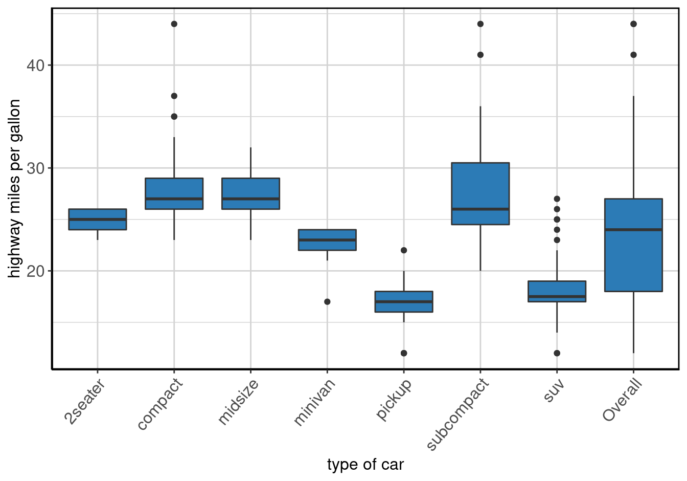
Figure 59: Boxplot of highway miles per gallon by type of car.
City MPG by Comments
The results are in table 79 and figure 60.
ctyByCommentsSummary <- data_summary(x = "cty", by = "comments", data = mpg)

make_complete_output(ctyByCommentsSummary)| some random comments | Label | N | P NA | Mean | S Dev | Med | MAD | 25th P | 75th P | IQR | Min | Max |
|---|---|---|---|---|---|---|---|---|---|---|---|---|
| . | city miles per gallon | 26 | 0 | 15.42 | 3.94 | 15.0 | 2.97 | 13 | 17 | 4.0 | 9 | 28 |
| Blah, Blah, Blah, Blah, Blah, Blah, Blah, Blah | city miles per gallon | 23 | 0 | 17.04 | 3.23 | 17.0 | 2.97 | 15 | 19 | 3.5 | 11 | 22 |
| Does it also fly? | city miles per gallon | 16 | 0 | 17.94 | 5.52 | 18.0 | 3.71 | 14 | 19 | 4.5 | 11 | 35 |
| Does it come in green? | city miles per gallon | 23 | 0 | 18.39 | 4.31 | 19.0 | 2.97 | 14 | 21 | 6.5 | 11 | 28 |
| I like this car! | city miles per gallon | 24 | 0 | 17.92 | 5.16 | 18.0 | 5.93 | 14 | 21 | 7.0 | 11 | 33 |
| Meh. | city miles per gallon | 18 | 0 | 16.33 | 3.40 | 16.0 | 3.71 | 14 | 19 | 4.5 | 11 | 25 |
| Missing | city miles per gallon | 25 | 0 | 15.84 | 5.16 | 15.0 | 4.45 | 12 | 19 | 7.0 | 9 | 26 |
| This is the worst car ever! | city miles per gallon | 22 | 0 | 17.09 | 4.00 | 18.0 | 4.45 | 14 | 19 | 4.5 | 9 | 26 |
| want cheese flavoured cars. | city miles per gallon | 33 | 0 | 16.91 | 3.95 | 16.0 | 2.97 | 14 | 20 | 6.0 | 11 | 29 |
| Overall | city miles per gallon | 234 | 0 | 16.86 | 4.26 | 17.0 | 4.45 | 14 | 19 | 5.0 | 9 | 35 |
| R NA Value | city miles per gallon | 24 | 0 | 16.17 | 3.34 | 15.5 | 3.71 | 14 | 19 | 5.0 | 11 | 22 |
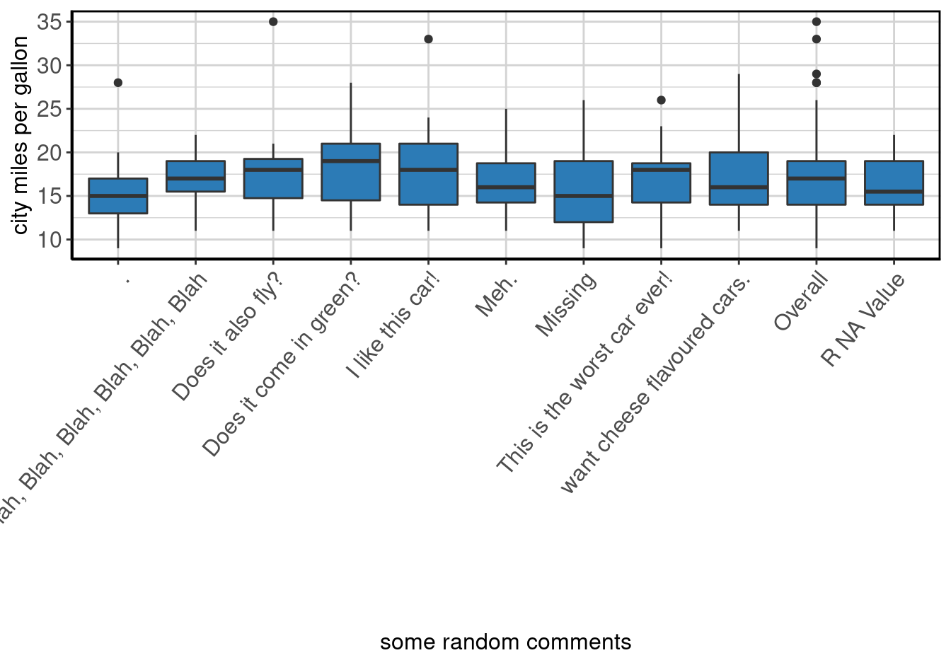
Figure 60: Boxplot of city miles per gallon by some random comments.
Highway MPG by Comments
The results are in table 80 and figure 61.
hwyByCommentsSummary <- data_summary(x = "hwy", by = "comments", data = mpg)

make_complete_output(hwyByCommentsSummary)| some random comments | Label | N | P NA | Mean | S Dev | Med | MAD | 25th P | 75th P | IQR | Min | Max |
|---|---|---|---|---|---|---|---|---|---|---|---|---|
| . | highway miles per gallon | 26 | 0 | 22.08 | 5.60 | 23.5 | 6.67 | 17 | 26 | 9.00 | 12 | 33 |
| Blah, Blah, Blah, Blah, Blah, Blah, Blah, Blah | highway miles per gallon | 23 | 0 | 24.09 | 4.95 | 26.0 | 4.45 | 20 | 29 | 8.50 | 15 | 31 |
| Does it also fly? | highway miles per gallon | 16 | 0 | 24.75 | 7.33 | 25.5 | 5.19 | 17 | 28 | 9.75 | 14 | 44 |
| Does it come in green? | highway miles per gallon | 23 | 0 | 25.26 | 5.50 | 27.0 | 4.45 | 19 | 29 | 9.50 | 16 | 37 |
| I like this car! | highway miles per gallon | 24 | 0 | 24.75 | 7.25 | 26.0 | 7.41 | 17 | 29 | 12.00 | 15 | 44 |
| Meh. | highway miles per gallon | 18 | 0 | 22.61 | 4.58 | 23.5 | 5.19 | 19 | 26 | 7.00 | 15 | 32 |
| Missing | highway miles per gallon | 25 | 0 | 21.96 | 7.33 | 19.0 | 5.93 | 17 | 26 | 9.00 | 12 | 36 |
| This is the worst car ever! | highway miles per gallon | 22 | 0 | 23.82 | 5.78 | 25.0 | 5.93 | 19 | 28 | 8.50 | 12 | 35 |
| want cheese flavoured cars. | highway miles per gallon | 33 | 0 | 23.33 | 5.85 | 24.0 | 7.41 | 17 | 27 | 10.00 | 15 | 41 |
| Overall | highway miles per gallon | 234 | 0 | 23.44 | 5.95 | 24.0 | 7.41 | 18 | 27 | 9.00 | 12 | 44 |
| R NA Value | highway miles per gallon | 24 | 0 | 22.33 | 4.72 | 24.0 | 5.19 | 17 | 25 | 7.50 | 15 | 31 |
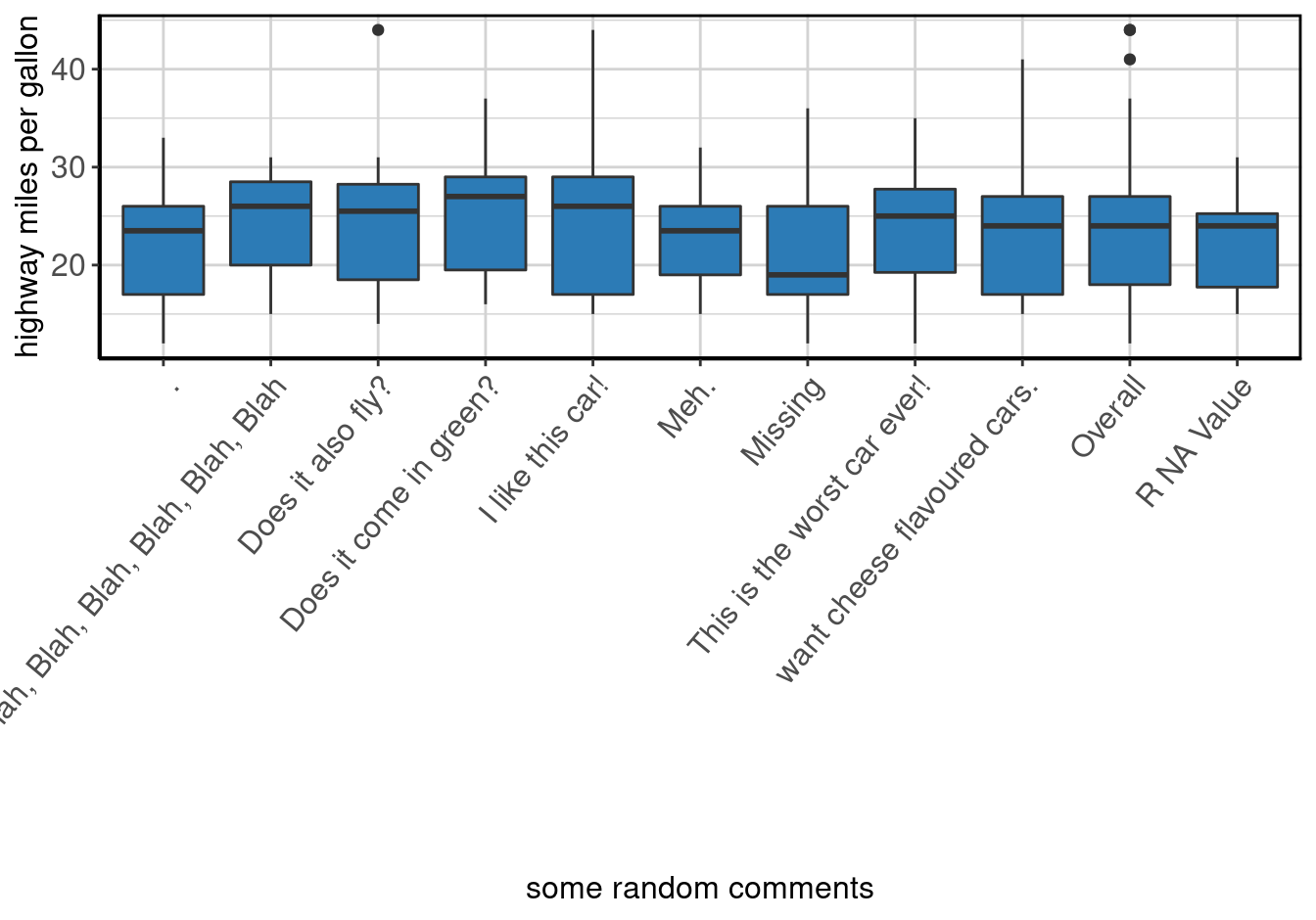
Figure 61: Boxplot of highway miles per gallon by some random comments.
City MPG by Party
The results are in table 81 and figure 62.
ctyByPartySummary <- data_summary(x = "cty", by = "party", data = mpg)

make_complete_output(ctyByPartySummary)| some random political parties | Label | N | P NA | Mean | S Dev | Med | MAD | 25th P | 75th P | IQR | Min | Max |
|---|---|---|---|---|---|---|---|---|---|---|---|---|
| republican | city miles per gallon | 56 | 0 | 17.29 | 4.52 | 17 | 5.19 | 14 | 21 | 7 | 9 | 29 |
| democrat | city miles per gallon | 61 | 0 | 16.26 | 4.59 | 16 | 4.45 | 13 | 19 | 6 | 9 | 33 |
| independent | city miles per gallon | 62 | 0 | 16.84 | 3.39 | 17 | 3.71 | 14 | 19 | 5 | 9 | 24 |
| Overall | city miles per gallon | 234 | 0 | 16.86 | 4.26 | 17 | 4.45 | 14 | 19 | 5 | 9 | 35 |
| R NA Value | city miles per gallon | 55 | 0 | 17.11 | 4.50 | 17 | 2.97 | 14 | 19 | 5 | 9 | 35 |
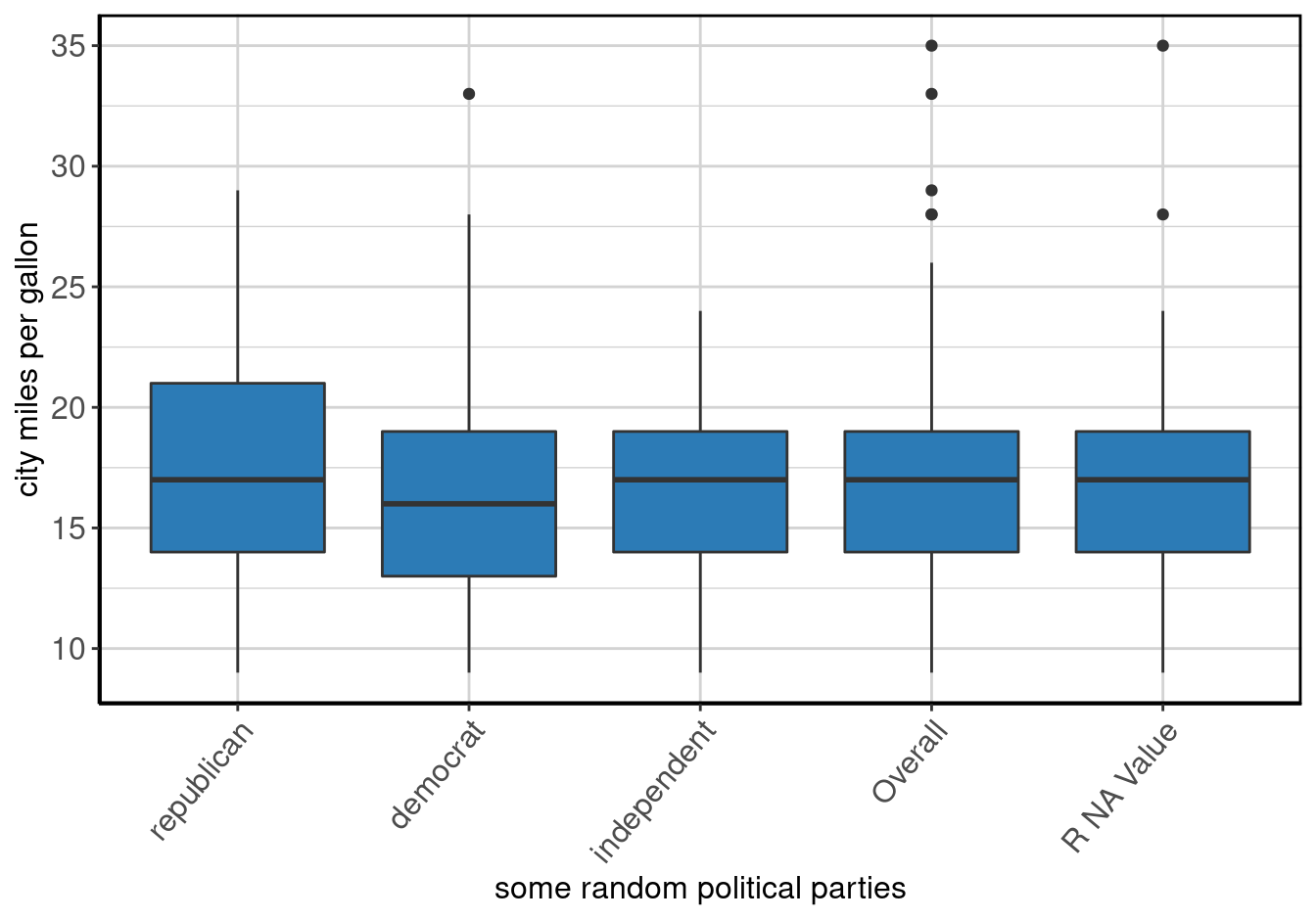
Figure 62: Boxplot of city miles per gallon by .
Highway MPG by Party
The results are in table 82 and figure 63.
hwyByPartySummary <- data_summary(x = "hwy", by = "party", data = mpg)

make_complete_output(hwyByPartySummary)| some random political parties | Label | N | P NA | Mean | S Dev | Med | MAD | 25th P | 75th P | IQR | Min | Max |
|---|---|---|---|---|---|---|---|---|---|---|---|---|
| republican | highway miles per gallon | 56 | 0 | 23.57 | 6.42 | 24 | 7.41 | 17 | 29 | 12 | 12 | 41 |
| democrat | highway miles per gallon | 61 | 0 | 22.38 | 6.25 | 21 | 7.41 | 17 | 27 | 10 | 12 | 44 |
| independent | highway miles per gallon | 62 | 0 | 23.68 | 4.83 | 25 | 4.45 | 19 | 27 | 8 | 12 | 36 |
| Overall | highway miles per gallon | 234 | 0 | 23.44 | 5.95 | 24 | 7.41 | 18 | 27 | 9 | 12 | 44 |
| R NA Value | highway miles per gallon | 55 | 0 | 24.22 | 6.26 | 26 | 4.45 | 18 | 28 | 10 | 12 | 44 |
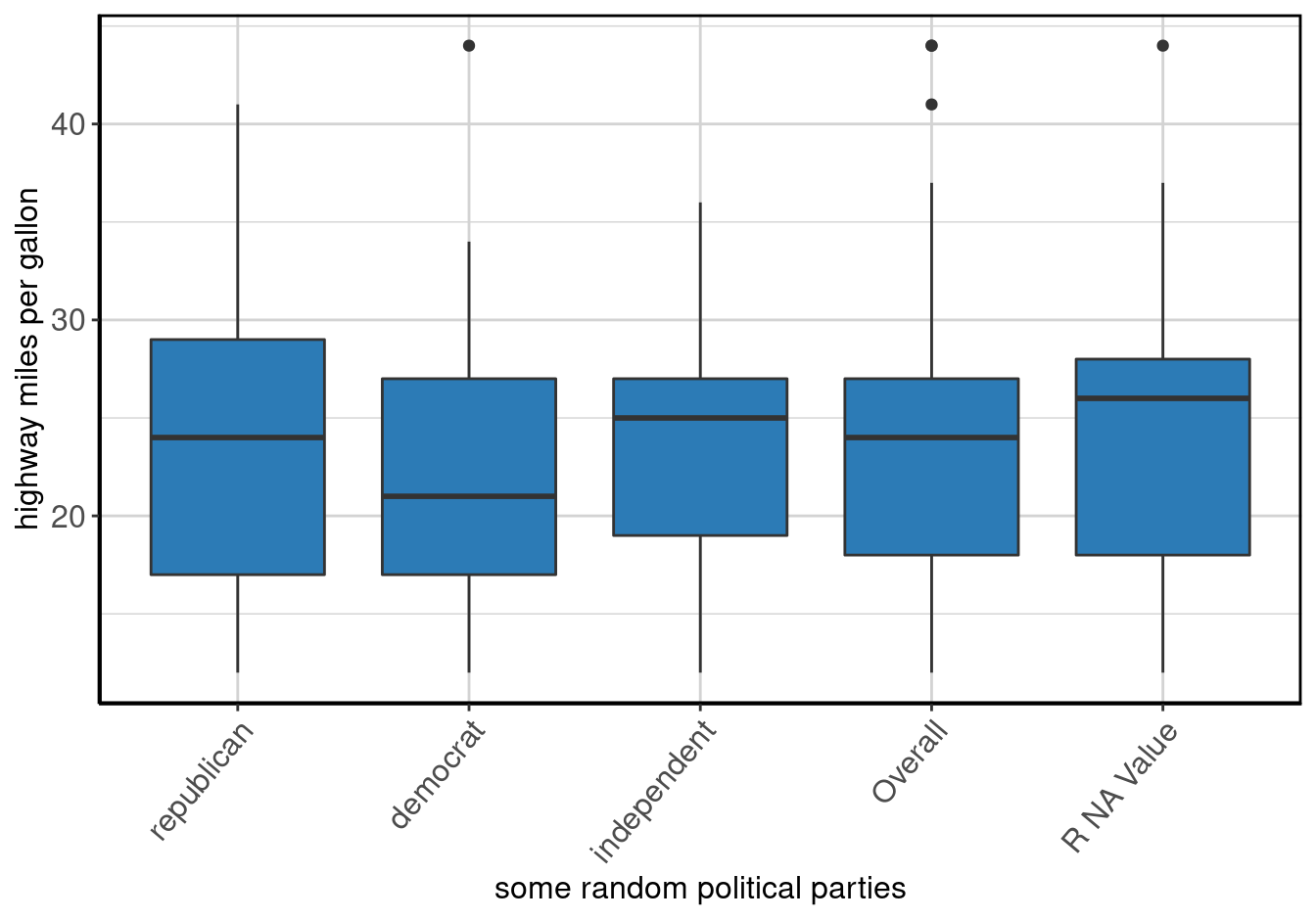
Figure 63: Boxplot of highway miles per gallon by .
City MPG by All Missing
The results are in table 83 and figure 64.
ctyByMissSummary <- data_summary(x = "cty", by = "miss", data = mpg)

make_complete_output(ctyByMissSummary)| an all missing variable | Label | N | P NA | Mean | S Dev | Med | MAD | 25th P | 75th P | IQR | Min | Max |
|---|---|---|---|---|---|---|---|---|---|---|---|---|
| Overall | city miles per gallon | 234 | 0 | 16.86 | 4.26 | 17 | 4.45 | 14 | 19 | 5 | 9 | 35 |
| R NA Value | city miles per gallon | 234 | 0 | 16.86 | 4.26 | 17 | 4.45 | 14 | 19 | 5 | 9 | 35 |
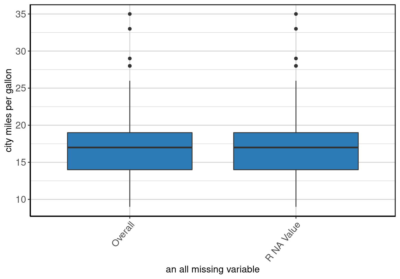
Figure 64: Boxplot of city miles per gallon by an all missing variable.
Highway MPG by All Missing
The results are in table 84 and figure 65.
hwyByMissSummary <- data_summary(x = "hwy", by = "miss", data = mpg)

make_complete_output(hwyByMissSummary)| an all missing variable | Label | N | P NA | Mean | S Dev | Med | MAD | 25th P | 75th P | IQR | Min | Max |
|---|---|---|---|---|---|---|---|---|---|---|---|---|
| Overall | highway miles per gallon | 234 | 0 | 23.44 | 5.95 | 24 | 7.41 | 18 | 27 | 9 | 12 | 44 |
| R NA Value | highway miles per gallon | 234 | 0 | 23.44 | 5.95 | 24 | 7.41 | 18 | 27 | 9 | 12 | 44 |
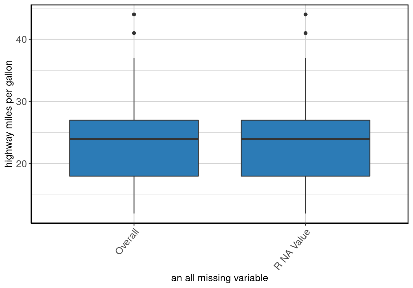
Figure 65: Boxplot of highway miles per gallon by an all missing variable.
Other Examples
Date of Purchase by Year of Manufacture
The results are in table 85 and figure 66.
dpByYearSummary <- data_summary(x = "dp", by = "year", data = mpg[which(mpg$dp != "1000-05-02" | is.na(mpg$dp)), ], difftime_units = "weeks")

make_complete_output(dpByYearSummary)| year of manufacture | Label | N | P NA | Mean | S Dev | Med | MAD | 25th P | 75th P | IQR | Min | Max |
|---|---|---|---|---|---|---|---|---|---|---|---|---|
| 1999 | date of purchase (Date class) | 107 | 8.55 | 1999-06-23 | 14.72 weeks | 1999-06-23 | 18.64 weeks | 1999-03-27 | 1999-10-13 | 28.57143 weeks | 1999-01-04 | 1999-12-24 |
| 2008 | date of purchase (Date class) | 106 | 8.62 | 2008-07-03 | 14.96 weeks | 2008-07-12 | 18.43 weeks | 2008-04-16 | 2008-10-18 | 26.42857 weeks | 2008-01-02 | 2008-12-23 |
| Overall | date of purchase (Date class) | 213 | 8.58 | 2003-12-21 | 236.59 weeks | 1999-12-24 | 74.98 weeks | 1999-07-14 | 2008-09-01 | 476.71429 weeks | 1999-01-04 | 2008-12-23 |
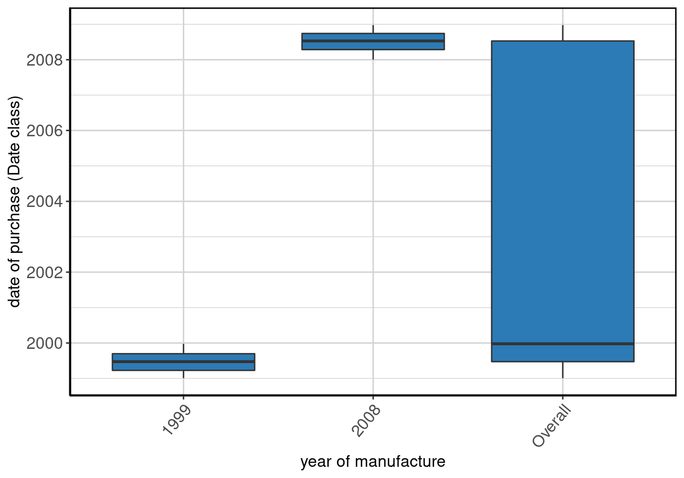
Figure 66: Boxplot of date of purchase (Date class) by year of manufacture.
Date of Purchase by Comments
The results are in table 86 and figure 67.
dpByCommentsSummary <- data_summary(x = "dp", by = "comments", data = mpg[which(mpg$dp != "1000-05-02" | is.na(mpg$dp)), ], difftime_units = "weeks")

make_complete_output(dpByCommentsSummary)| some random comments | Label | N | P NA | Mean | S Dev | Med | MAD | 25th P | 75th P | IQR | Min | Max |
|---|---|---|---|---|---|---|---|---|---|---|---|---|
| . | date of purchase (Date class) | 25 | 3.85 | 2004-08-08 | 237.07 weeks | 2008-02-08 | 60.57 weeks | 1999-09-19 | 2008-09-06 | 467.8571 weeks | 1999-01-13 | 2008-11-27 |
| Blah, Blah, Blah, Blah, Blah, Blah, Blah, Blah | date of purchase (Date class) | 21 | 8.70 | 2003-10-28 | 243.86 weeks | 1999-12-14 | 66.51 weeks | 1999-06-28 | 2008-08-02 | 474.7143 weeks | 1999-02-03 | 2008-12-23 |
| Does it also fly? | date of purchase (Date class) | 13 | 18.75 | 2002-12-21 | 240.09 weeks | 1999-10-13 | 52.31 weeks | 1999-07-03 | 2008-11-10 | 488.2857 weeks | 1999-01-14 | 2008-11-26 |
| Does it come in green? | date of purchase (Date class) | 23 | 0.00 | 2004-01-22 | 241.15 weeks | 2008-01-04 | 71.80 weeks | 1999-04-26 | 2008-03-24 | 465.0000 weeks | 1999-01-16 | 2008-12-08 |
| I like this car! | date of purchase (Date class) | 20 | 13.04 | 2003-08-29 | 246.12 weeks | 1999-11-13 | 54.96 weeks | 1999-06-23 | 2008-09-23 | 482.8571 weeks | 1999-02-12 | 2008-12-15 |
| Meh. | date of purchase (Date class) | 17 | 5.56 | 2004-02-12 | 243.37 weeks | 2008-01-27 | 51.47 weeks | 1999-04-04 | 2008-05-27 | 477.2857 weeks | 1999-01-05 | 2008-09-26 |
| Missing | date of purchase (Date class) | 22 | 12.00 | 2005-03-23 | 234.82 weeks | 2008-03-25 | 44.90 weeks | 1999-08-24 | 2008-10-11 | 476.5714 weeks | 1999-01-04 | 2008-11-15 |
| This is the worst car ever! | date of purchase (Date class) | 21 | 4.55 | 2003-11-06 | 240.62 weeks | 1999-11-24 | 52.31 weeks | 1999-06-27 | 2008-07-17 | 472.5714 weeks | 1999-03-22 | 2008-10-26 |
| want cheese flavoured cars. | date of purchase (Date class) | 31 | 6.06 | 2003-04-02 | 235.66 weeks | 1999-12-06 | 58.46 weeks | 1999-05-07 | 2008-06-24 | 476.5714 weeks | 1999-01-26 | 2008-12-09 |
| Overall | date of purchase (Date class) | 213 | 8.58 | 2003-12-21 | 236.59 weeks | 1999-12-24 | 74.98 weeks | 1999-07-14 | 2008-09-01 | 476.7143 weeks | 1999-01-04 | 2008-12-23 |
| R NA Value | date of purchase (Date class) | 20 | 16.67 | 2003-12-06 | 236.95 weeks | 2003-12-24 | 337.72 weeks | 1999-08-14 | 2008-06-25 | 462.5714 weeks | 1999-01-07 | 2008-12-03 |
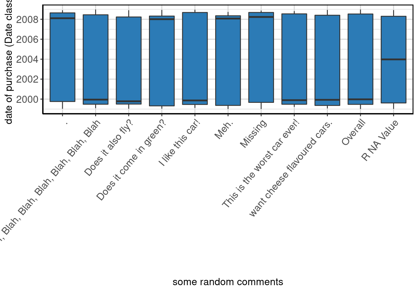
Figure 67: Boxplot of date of purchase (Date class) by some random comments.
Random Number by Party
The results are in table 87 and figure 68.
rnByPartySummary <- data_summary(x = "rn", by = "party", data = mpg)

make_complete_output(rnByPartySummary)| some random political parties | Label | N | P NA | Mean | S Dev | Med | MAD | 25th P | 75th P | IQR | Min | Max |
|---|---|---|---|---|---|---|---|---|---|---|---|---|
| republican | some random numbers that are generated from a normal distrubtion with mean = 10 and sd = 5 | 41 | 26.79 | 10.39 | 6.15 | 11.78 | 4.28 | 5.67 | 13.95 | 8.28 | -0.19 | 22.88 |
| democrat | some random numbers that are generated from a normal distrubtion with mean = 10 and sd = 5 | 46 | 24.59 | 10.00 | 5.37 | 10.41 | 5.38 | 6.34 | 13.24 | 6.74 | -2.54 | 23.46 |
| independent | some random numbers that are generated from a normal distrubtion with mean = 10 and sd = 5 | 54 | 12.90 | 10.60 | 4.99 | 10.49 | 5.46 | 7.12 | 14.52 | 7.25 | 0.74 | 20.81 |
| Overall | some random numbers that are generated from a normal distrubtion with mean = 10 and sd = 5 | 184 | 21.37 | 10.53 | 5.09 | 10.73 | 4.72 | 7.12 | 13.32 | 6.12 | -2.54 | 23.46 |
| R NA Value | some random numbers that are generated from a normal distrubtion with mean = 10 and sd = 5 | 43 | 21.82 | 11.16 | 3.71 | 10.72 | 2.65 | 8.99 | 12.81 | 3.72 | 4.42 | 22.44 |
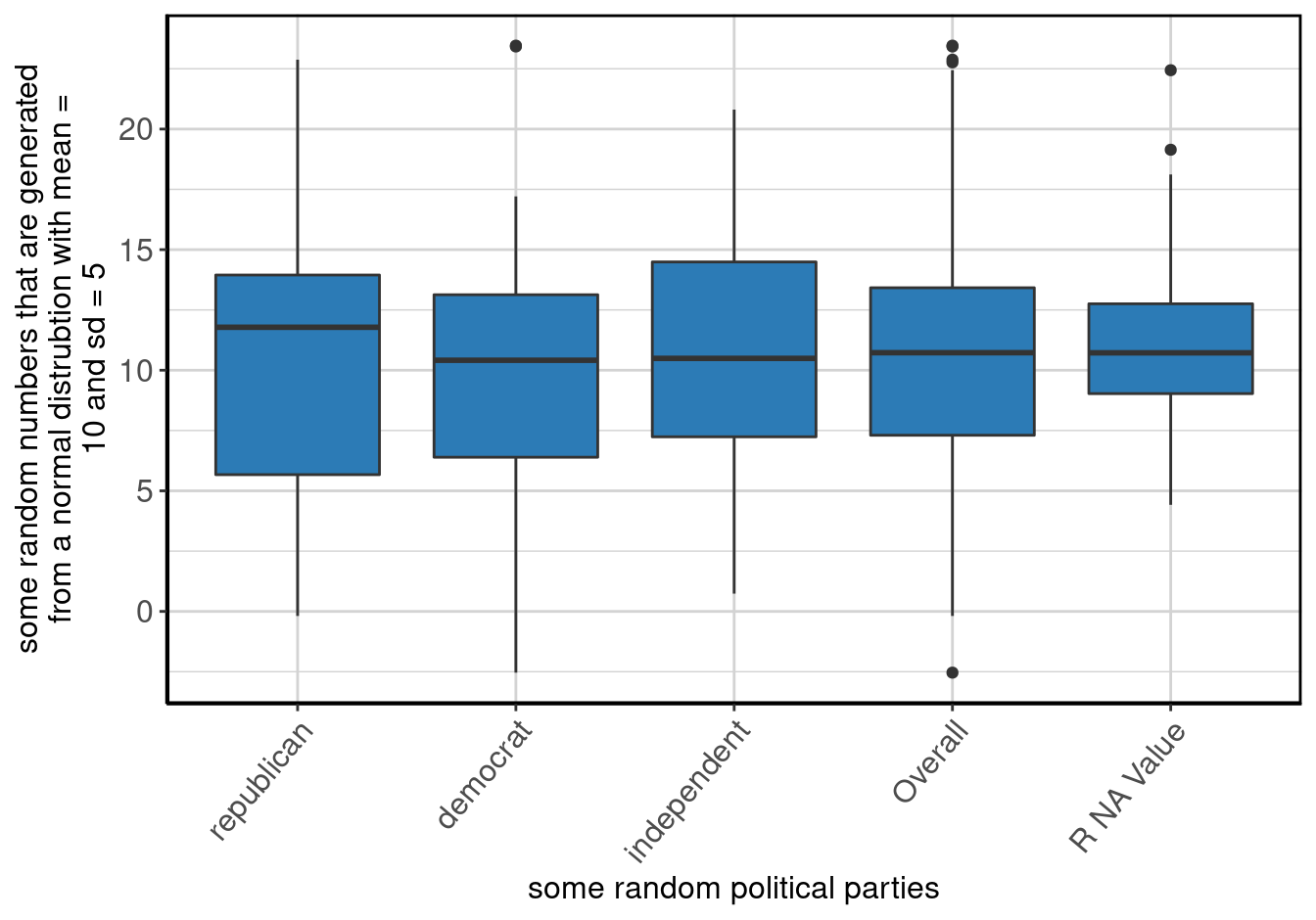
Figure 68: Boxplot of some random numbers that are generated from a normal distrubtion with mean = 10 and sd = 5 by some random political parties.
Random Difference in Time by Party
The results are in table 88 and figure 69.
rdifftimeByPartySummary <- data_summary(x = "rdifftime", by = "party", difftime_units = "weeks", data = mpg)

make_complete_output(rdifftimeByPartySummary)| some random political parties | Label | N | P NA | Mean | S Dev | Med | MAD | 25th P | 75th P | IQR | Min | Max |
|---|---|---|---|---|---|---|---|---|---|---|---|---|
| republican | some random numbers that are generated from a normal distrubtion with mean = 10 and sd = 5, and then converted to weeks | 45 | 19.64 | 9.50 weeks | 5.91 weeks | 10.35 weeks | 6.54 weeks | 4.96 weeks | 13.06 weeks | 8.11 weeks | 0.00 weeks | 23.49 weeks |
| democrat | some random numbers that are generated from a normal distrubtion with mean = 10 and sd = 5, and then converted to weeks | 52 | 14.75 | 9.31 weeks | 4.49 weeks | 9.38 weeks | 4.37 weeks | 6.44 weeks | 12.68 weeks | 6.23 weeks | 0.00 weeks | 18.28 weeks |
| independent | some random numbers that are generated from a normal distrubtion with mean = 10 and sd = 5, and then converted to weeks | 47 | 24.19 | 10.22 weeks | 4.64 weeks | 9.58 weeks | 5.87 weeks | 5.61 weeks | 13.57 weeks | 7.64 weeks | 2.04 weeks | 21.65 weeks |
| Overall | some random numbers that are generated from a normal distrubtion with mean = 10 and sd = 5, and then converted to weeks | 184 | 21.37 | 9.76 weeks | 5.07 weeks | 9.60 weeks | 5.12 weeks | 6.11 weeks | 13.05 weeks | 6.79 weeks | 0.00 weeks | 23.49 weeks |
| R NA Value | some random numbers that are generated from a normal distrubtion with mean = 10 and sd = 5, and then converted to weeks | 40 | 27.27 | 10.08 weeks | 5.38 weeks | 10.06 weeks | 4.12 weeks | 6.76 weeks | 12.27 weeks | 5.46 weeks | 0.00 weeks | 22.98 weeks |
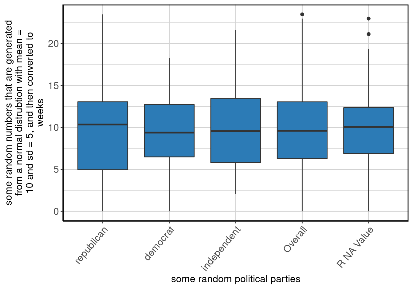
Figure 69: Boxplot of some random numbers that are generated from a normal distrubtion with mean = 10 and sd = 5, and then converted to weeks by some random political parties.
Random Difference in Time by Comments
The results are in table 89 and figure 70.
rdifftimeByCommentsSummary <- data_summary(x = "rdifftime", by = "comments", difftime_units = "weeks", data = mpg)

make_complete_output(rdifftimeByCommentsSummary)| some random comments | Label | N | P NA | Mean | S Dev | Med | MAD | 25th P | 75th P | IQR | Min | Max |
|---|---|---|---|---|---|---|---|---|---|---|---|---|
| . | some random numbers that are generated from a normal distrubtion with mean = 10 and sd = 5, and then converted to weeks | 21 | 19.23 | 8.21 weeks | 5.55 weeks | 9.07 weeks | 5.97 weeks | 4.81 weeks | 10.97 weeks | 6.16 weeks | 0.00 weeks | 19.07 weeks |
| Blah, Blah, Blah, Blah, Blah, Blah, Blah, Blah | some random numbers that are generated from a normal distrubtion with mean = 10 and sd = 5, and then converted to weeks | 19 | 17.39 | 8.32 weeks | 4.50 weeks | 9.57 weeks | 3.78 weeks | 4.33 weeks | 11.54 weeks | 6.86 weeks | 0.00 weeks | 14.76 weeks |
| Does it also fly? | some random numbers that are generated from a normal distrubtion with mean = 10 and sd = 5, and then converted to weeks | 14 | 12.50 | 9.49 weeks | 5.54 weeks | 10.25 weeks | 4.60 weeks | 6.51 weeks | 13.29 weeks | 6.34 weeks | 0.00 weeks | 21.14 weeks |
| Does it come in green? | some random numbers that are generated from a normal distrubtion with mean = 10 and sd = 5, and then converted to weeks | 19 | 17.39 | 8.51 weeks | 4.28 weeks | 8.76 weeks | 4.49 weeks | 5.27 weeks | 11.79 weeks | 5.44 weeks | 0.00 weeks | 16.31 weeks |
| I like this car! | some random numbers that are generated from a normal distrubtion with mean = 10 and sd = 5, and then converted to weeks | 22 | 8.33 | 10.44 weeks | 6.03 weeks | 9.78 weeks | 6.78 weeks | 5.32 weeks | 16.22 weeks | 10.30 weeks | 1.79 weeks | 21.65 weeks |
| Meh. | some random numbers that are generated from a normal distrubtion with mean = 10 and sd = 5, and then converted to weeks | 13 | 27.78 | 10.21 weeks | 4.88 weeks | 10.56 weeks | 4.61 weeks | 7.13 weeks | 12.60 weeks | 5.47 weeks | 3.88 weeks | 21.71 weeks |
| Missing | some random numbers that are generated from a normal distrubtion with mean = 10 and sd = 5, and then converted to weeks | 19 | 24.00 | 11.44 weeks | 5.29 weeks | 12.24 weeks | 5.19 weeks | 6.65 weeks | 15.38 weeks | 8.17 weeks | 3.57 weeks | 23.49 weeks |
| This is the worst car ever! | some random numbers that are generated from a normal distrubtion with mean = 10 and sd = 5, and then converted to weeks | 17 | 22.73 | 9.28 weeks | 4.29 weeks | 9.63 weeks | 4.80 weeks | 6.76 weeks | 13.05 weeks | 6.29 weeks | 0.36 weeks | 13.93 weeks |
| want cheese flavoured cars. | some random numbers that are generated from a normal distrubtion with mean = 10 and sd = 5, and then converted to weeks | 26 | 21.21 | 10.88 weeks | 3.62 weeks | 11.19 weeks | 3.00 weeks | 9.01 weeks | 13.16 weeks | 3.91 weeks | 2.53 weeks | 17.07 weeks |
| Overall | some random numbers that are generated from a normal distrubtion with mean = 10 and sd = 5, and then converted to weeks | 184 | 21.37 | 9.76 weeks | 5.07 weeks | 9.60 weeks | 5.12 weeks | 6.11 weeks | 13.05 weeks | 6.79 weeks | 0.00 weeks | 23.49 weeks |
| R NA Value | some random numbers that are generated from a normal distrubtion with mean = 10 and sd = 5, and then converted to weeks | 14 | 41.67 | 10.69 weeks | 6.75 weeks | 11.80 weeks | 7.16 weeks | 5.23 weeks | 15.02 weeks | 9.42 weeks | 0.00 weeks | 22.98 weeks |
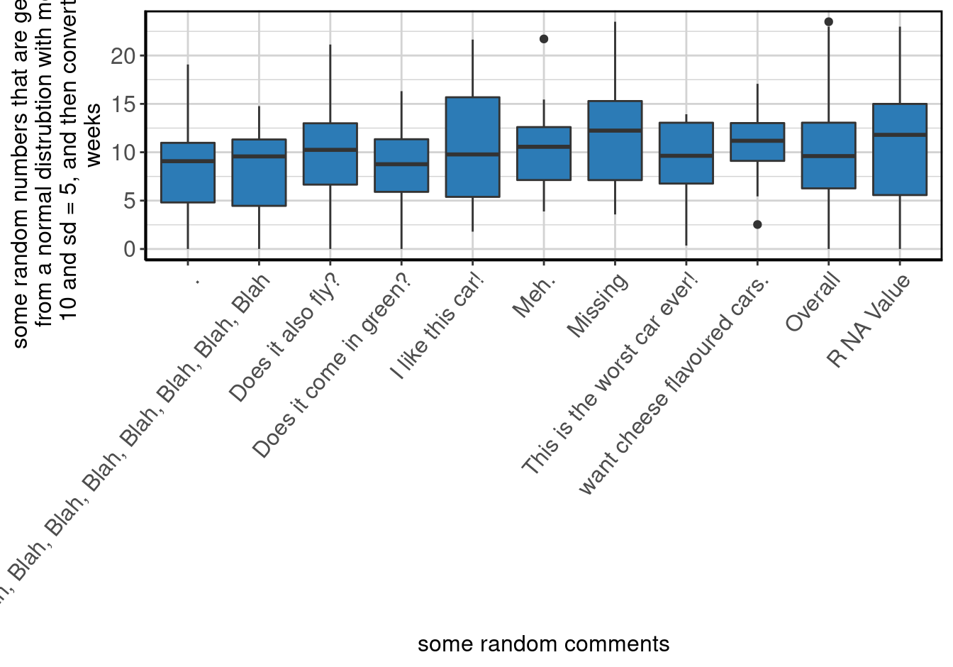
Figure 70: Boxplot of some random numbers that are generated from a normal distrubtion with mean = 10 and sd = 5, and then converted to weeks by some random comments.
Comments by Party
The results are in table 90 and figure 71.
commentsByPartySummary <- data_summary(x = "comments", by = "party", data = mpg)

make_complete_output(commentsByPartySummary)| some random comments | republican | democrat | independent | Overall | R NA Value |
|---|---|---|---|---|---|
| . | 3 (5.36%) | 7 (11.48%) | 9 (14.52%) | 26 (11.11%) | 7 (12.73%) |
| Blah, Blah, Blah, Blah, Blah, Blah, Blah, Blah | 5 (8.93%) | 7 (11.48%) | 6 (9.68%) | 23 (9.83%) | 5 (9.09%) |
| Does it also fly? | 1 (1.79%) | 6 (9.84%) | 3 (4.84%) | 16 (6.84%) | 6 (10.91%) |
| Does it come in green? | 8 (14.29%) | 6 (9.84%) | 6 (9.68%) | 23 (9.83%) | 3 (5.45%) |
| I like this car! | 6 (10.71%) | 6 (9.84%) | 8 (12.9%) | 24 (10.26%) | 4 (7.27%) |
| Meh. | 10 (17.86%) | 5 (8.2%) | 0 (0%) | 18 (7.69%) | 3 (5.45%) |
| Missing | 5 (8.93%) | 9 (14.75%) | 6 (9.68%) | 25 (10.68%) | 5 (9.09%) |
| This is the worst car ever! | 9 (16.07%) | 4 (6.56%) | 4 (6.45%) | 22 (9.4%) | 5 (9.09%) |
| want cheese flavoured cars. | 7 (12.5%) | 7 (11.48%) | 10 (16.13%) | 33 (14.1%) | 9 (16.36%) |
| R NA Value | 2 (3.57%) | 4 (6.56%) | 10 (16.13%) | 24 (10.26%) | 8 (14.55%) |
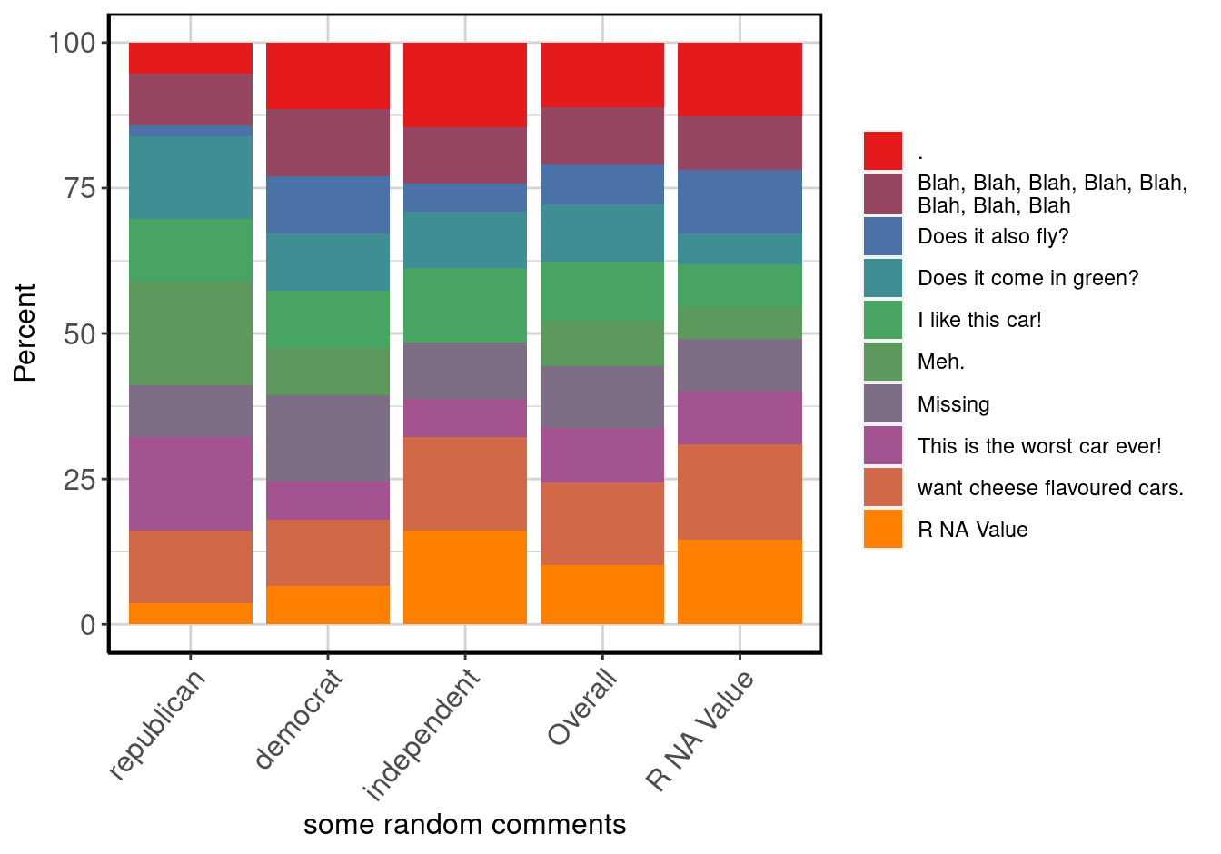
Figure 71: Barplot of some random comments by some random political parties.
By By Data Summaries
City MPG by Number of Cylinders by Class
The results are in table 69 and figure 50.
ctyByCylByClassSummary <- data_summary(x = "cty", by = c("cyl", "class"), data = mpg)

make_complete_output(ctyByCylByClassSummary)| number of cylinders by type of car | Label | N | P NA | Mean | S Dev | Med | MAD | 25th P | 75th P | IQR | Min | Max |
|---|---|---|---|---|---|---|---|---|---|---|---|---|
| 8, 2seater | city miles per gallon | 5 | 0 | 15.40 | 0.55 | 15.0 | 0.00 | 15 | 16 | 1.00 | 15 | 16 |
| 4, compact | city miles per gallon | 32 | 0 | 21.38 | 3.25 | 21.0 | 1.48 | 19 | 22 | 2.25 | 16 | 33 |
| 5, compact | city miles per gallon | 2 | 0 | 21.00 | 0.00 | 21.0 | 0.00 | 21 | 21 | 0.00 | 21 | 21 |
| 6, compact | city miles per gallon | 13 | 0 | 16.92 | 1.12 | 17.0 | 1.48 | 16 | 18 | 2.00 | 15 | 18 |
| 4, midsize | city miles per gallon | 16 | 0 | 20.50 | 1.63 | 21.0 | 0.74 | 19 | 21 | 2.00 | 18 | 23 |
| 6, midsize | city miles per gallon | 23 | 0 | 17.78 | 1.09 | 18.0 | 1.48 | 17 | 19 | 1.50 | 15 | 19 |
| 8, midsize | city miles per gallon | 2 | 0 | 16.00 | 0.00 | 16.0 | 0.00 | 16 | 16 | 0.00 | 16 | 16 |
| 4, minivan | city miles per gallon | 1 | 0 | 18.00 | NA | 18.0 | 0.00 | 18 | 18 | 0.00 | 18 | 18 |
| 6, minivan | city miles per gallon | 10 | 0 | 15.60 | 1.78 | 16.0 | 1.48 | 15 | 17 | 1.50 | 11 | 17 |
| 4, pickup | city miles per gallon | 3 | 0 | 16.00 | 1.00 | 16.0 | 1.48 | 15 | 17 | 1.00 | 15 | 17 |
| 6, pickup | city miles per gallon | 10 | 0 | 14.50 | 0.85 | 14.5 | 0.74 | 14 | 15 | 1.00 | 13 | 16 |
| 8, pickup | city miles per gallon | 20 | 0 | 11.80 | 1.58 | 12.0 | 1.48 | 11 | 13 | 2.00 | 9 | 14 |
| 4, subcompact | city miles per gallon | 21 | 0 | 22.86 | 4.19 | 21.0 | 2.97 | 19 | 25 | 6.00 | 19 | 35 |
| 5, subcompact | city miles per gallon | 2 | 0 | 20.00 | 0.00 | 20.0 | 0.00 | 20 | 20 | 0.00 | 20 | 20 |
| 6, subcompact | city miles per gallon | 7 | 0 | 17.00 | 0.82 | 17.0 | 1.48 | 16 | 18 | 1.00 | 16 | 18 |
| 8, subcompact | city miles per gallon | 5 | 0 | 14.80 | 0.45 | 15.0 | 0.00 | 15 | 15 | 0.00 | 14 | 15 |
| 4, suv | city miles per gallon | 8 | 0 | 18.00 | 1.77 | 18.0 | 2.22 | 16 | 19 | 1.75 | 15 | 20 |
| 6, suv | city miles per gallon | 16 | 0 | 14.50 | 1.10 | 14.5 | 0.74 | 14 | 15 | 1.00 | 13 | 17 |
| 8, suv | city miles per gallon | 38 | 0 | 12.13 | 1.36 | 12.0 | 1.48 | 11 | 13 | 2.00 | 9 | 14 |
| Overall | city miles per gallon | 234 | 0 | 16.86 | 4.26 | 17.0 | 4.45 | 14 | 19 | 5.00 | 9 | 35 |
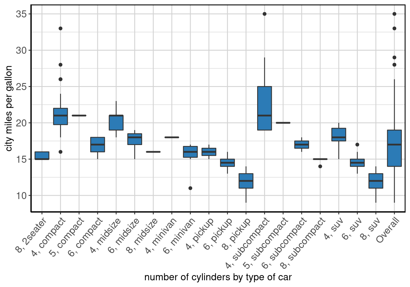
Figure 72: Boxplot of city miles per gallon by number of cylinders by type of car.
Highway MPG by Number of Cylinders by Class
The results are in table 70 and figure 51.
hwyByCylByClassSummary <- data_summary(x = "hwy", by = c("cyl", "class"), data = mpg)

make_complete_output(hwyByCylByClassSummary)| number of cylinders by type of car | Label | N | P NA | Mean | S Dev | Med | MAD | 25th P | 75th P | IQR | Min | Max |
|---|---|---|---|---|---|---|---|---|---|---|---|---|
| 8, 2seater | highway miles per gallon | 5 | 0 | 24.80 | 1.30 | 25.0 | 1.48 | 24 | 26 | 2.00 | 23 | 26 |
| 4, compact | highway miles per gallon | 32 | 0 | 29.47 | 3.93 | 29.0 | 2.97 | 27 | 30 | 3.25 | 25 | 44 |
| 5, compact | highway miles per gallon | 2 | 0 | 29.00 | 0.00 | 29.0 | 0.00 | 29 | 29 | 0.00 | 29 | 29 |
| 6, compact | highway miles per gallon | 13 | 0 | 25.31 | 1.18 | 25.0 | 1.48 | 25 | 26 | 1.00 | 23 | 27 |
| 4, midsize | highway miles per gallon | 16 | 0 | 29.19 | 1.80 | 29.0 | 2.97 | 27 | 31 | 3.25 | 26 | 32 |
| 6, midsize | highway miles per gallon | 23 | 0 | 26.26 | 1.14 | 26.0 | 0.00 | 26 | 27 | 0.50 | 24 | 29 |
| 8, midsize | highway miles per gallon | 2 | 0 | 24.00 | 1.41 | 24.0 | 1.48 | 23 | 25 | 1.00 | 23 | 25 |
| 4, minivan | highway miles per gallon | 1 | 0 | 24.00 | NA | 24.0 | 0.00 | 24 | 24 | 0.00 | 24 | 24 |
| 6, minivan | highway miles per gallon | 10 | 0 | 22.20 | 2.10 | 22.5 | 1.48 | 22 | 24 | 1.75 | 17 | 24 |
| 4, pickup | highway miles per gallon | 3 | 0 | 20.67 | 1.15 | 20.0 | 0.00 | 20 | 22 | 1.00 | 20 | 22 |
| 6, pickup | highway miles per gallon | 10 | 0 | 17.90 | 1.10 | 17.5 | 0.74 | 17 | 19 | 1.75 | 17 | 20 |
| 8, pickup | highway miles per gallon | 20 | 0 | 15.80 | 1.99 | 16.0 | 1.48 | 15 | 17 | 2.00 | 12 | 19 |
| 4, subcompact | highway miles per gallon | 21 | 0 | 30.81 | 5.12 | 29.0 | 4.45 | 26 | 33 | 7.00 | 26 | 44 |
| 5, subcompact | highway miles per gallon | 2 | 0 | 28.50 | 0.71 | 28.5 | 0.74 | 28 | 29 | 0.50 | 28 | 29 |
| 6, subcompact | highway miles per gallon | 7 | 0 | 24.71 | 0.95 | 24.0 | 0.00 | 24 | 26 | 1.50 | 24 | 26 |
| 8, subcompact | highway miles per gallon | 5 | 0 | 21.60 | 1.14 | 22.0 | 1.48 | 21 | 22 | 1.00 | 20 | 23 |
| 4, suv | highway miles per gallon | 8 | 0 | 23.75 | 2.60 | 24.5 | 2.22 | 20 | 25 | 3.00 | 20 | 27 |
| 6, suv | highway miles per gallon | 16 | 0 | 18.50 | 1.55 | 19.0 | 2.22 | 17 | 19 | 2.25 | 17 | 22 |
| 8, suv | highway miles per gallon | 38 | 0 | 16.79 | 1.91 | 17.0 | 1.48 | 15 | 18 | 2.75 | 12 | 20 |
| Overall | highway miles per gallon | 234 | 0 | 23.44 | 5.95 | 24.0 | 7.41 | 18 | 27 | 9.00 | 12 | 44 |
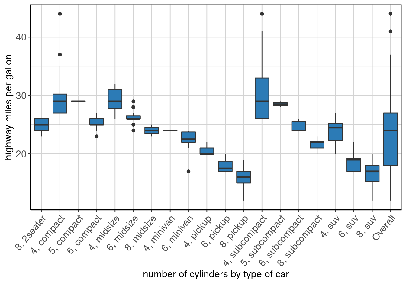
Figure 73: Boxplot of highway miles per gallon by number of cylinders by type of car.
Date of Purchase of Cylinders by Comments
The results are in table 93 and figure 74.
dpByCylByCommentsSummary <- data_summary(x = "dp", by = c("cyl", "comments"), difftime_units = "weeks", data = mpg[which(mpg$dp != "1000-05-02" | is.na(mpg$dp)), ])

make_complete_output(dpByCylByCommentsSummary)| number of cylinders by some random comments | Label | N | P NA | Mean | S Dev | Med | MAD | 25th P | 75th P | IQR | Min | Max |
|---|---|---|---|---|---|---|---|---|---|---|---|---|
| 4, . | date of purchase (Date class) | 5 | 0.00 | 2003-01-27 | 252.39 weeks | 1999-10-26 | 54.64 weeks | 1999-02-10 | 2008-02-08 | 469.285714 weeks | 1999-02-10 | 2008-08-12 |
| 6, . | date of purchase (Date class) | 9 | 0.00 | 2004-08-21 | 241.15 weeks | 2008-04-02 | 44.27 weeks | 1999-08-28 | 2008-06-18 | 459.571429 weeks | 1999-07-14 | 2008-10-28 |
| 8, . | date of purchase (Date class) | 10 | 9.09 | 2004-11-28 | 246.03 weeks | 2008-02-07 | 61.53 weeks | 1999-10-05 | 2008-09-06 | 465.571429 weeks | 1999-01-13 | 2008-11-27 |
| 4, Blah, Blah, Blah, Blah, Blah, Blah, Blah, Blah | date of purchase (Date class) | 9 | 0.00 | 2002-08-10 | 241.71 weeks | 1999-09-12 | 38.34 weeks | 1999-03-15 | 2008-05-25 | 479.857143 weeks | 1999-03-08 | 2008-12-23 |
| 6, Blah, Blah, Blah, Blah, Blah, Blah, Blah, Blah | date of purchase (Date class) | 7 | 12.50 | 2004-08-16 | 254.96 weeks | 2008-05-13 | 31.13 weeks | 1999-06-07 | 2008-08-02 | 477.714286 weeks | 1999-03-19 | 2008-10-07 |
| 8, Blah, Blah, Blah, Blah, Blah, Blah, Blah, Blah | date of purchase (Date class) | 4 | 0.00 | 2004-01-07 | 274.68 weeks | 2004-02-23 | 342.16 weeks | 1999-02-03 | 2008-06-12 | 488.142857 weeks | 1999-02-03 | 2008-09-09 |
| 4, Does it also fly? | date of purchase (Date class) | 5 | 0.00 | 2002-12-14 | 265.47 weeks | 1999-08-06 | 43.21 weeks | 1999-01-14 | 2008-02-14 | 474.000000 weeks | 1999-01-14 | 2008-11-26 |
| 6, Does it also fly? | date of purchase (Date class) | 4 | 42.86 | 2001-09-28 | 225.84 weeks | 1999-08-23 | 12.71 weeks | 1999-07-03 | NA | NA weeks | 1999-06-15 | 2008-03-25 |
| 8, Does it also fly? | date of purchase (Date class) | 4 | 0.00 | 2004-03-25 | 272.68 weeks | 2004-04-06 | 347.46 weeks | 1999-07-16 | 2008-08-25 | 475.428571 weeks | 1999-07-16 | 2008-11-10 |
| 4, Does it come in green? | date of purchase (Date class) | 15 | 0.00 | 2003-07-23 | 243.88 weeks | 1999-08-26 | 47.02 weeks | 1999-03-24 | 2008-02-26 | 465.857143 weeks | 1999-01-16 | 2008-10-13 |
| 6, Does it come in green? | date of purchase (Date class) | 3 | 0.00 | 2002-06-23 | 268.42 weeks | 1999-09-09 | 27.75 weeks | 1999-05-01 | 1999-09-09 | 18.714286 weeks | 1999-05-01 | 2008-05-31 |
| 8, Does it come in green? | date of purchase (Date class) | 5 | 0.00 | 2006-07-09 | 217.62 weeks | 2008-02-09 | 24.15 weeks | 1999-02-01 | 2008-06-02 | 487.000000 weeks | 1999-02-01 | 2008-12-08 |
| 4, I like this car! | date of purchase (Date class) | 8 | 11.11 | 2005-04-06 | 247.72 weeks | 2008-07-29 | 20.33 weeks | 1999-06-23 | 2008-09-23 | 482.857143 weeks | 1999-06-08 | 2008-12-12 |
| 6, I like this car! | date of purchase (Date class) | 7 | 22.22 | 2002-01-30 | 232.78 weeks | 1999-08-23 | 25.84 weeks | 1999-04-23 | 2008-09-05 | 489.000000 weeks | 1999-03-13 | 2008-09-05 |
| 8, I like this car! | date of purchase (Date class) | 4 | 0.00 | 2001-11-20 | 246.39 weeks | 1999-09-27 | 30.61 weeks | 1999-02-12 | 1999-11-28 | 41.285714 weeks | 1999-02-12 | 2008-12-14 |
| 4, Meh. | date of purchase (Date class) | 6 | 0.00 | 1999-05-01 | 9.86 weeks | 1999-04-25 | 8.47 weeks | 1999-03-26 | 1999-05-16 | 7.285714 weeks | 1999-01-25 | 1999-08-11 |
| 6, Meh. | date of purchase (Date class) | 6 | 0.00 | 2005-06-05 | 248.14 weeks | 2008-04-27 | 26.58 weeks | 1999-07-31 | 2008-05-08 | 457.714286 weeks | 1999-01-05 | 2008-09-26 |
| 8, Meh. | date of purchase (Date class) | 5 | 16.67 | 2008-04-14 | 9.80 weeks | 2008-04-15 | 11.44 weeks | 2008-02-21 | 2008-05-27 | 13.714286 weeks | 2008-01-27 | 2008-07-13 |
| 4, Missing | date of purchase (Date class) | 3 | 50.00 | 2002-08-26 | 280.92 weeks | 1999-10-09 | 34.74 weeks | 1999-10-09 | NA | NA weeks | 1999-04-28 | 2008-11-11 |
| 6, Missing | date of purchase (Date class) | 5 | 0.00 | 2004-12-23 | 255.73 weeks | 2008-05-24 | 21.18 weeks | 1999-07-30 | 2008-08-09 | 471.142857 weeks | 1999-07-30 | 2008-09-01 |
| 8, Missing | date of purchase (Date class) | 14 | 0.00 | 2005-11-13 | 226.66 weeks | 2008-04-02 | 38.55 weeks | 1999-10-04 | 2008-09-08 | 466.000000 weeks | 1999-01-04 | 2008-11-15 |
| 4, This is the worst car ever! | date of purchase (Date class) | 7 | 0.00 | 2003-05-28 | 247.48 weeks | 1999-11-24 | 50.62 weeks | 1999-06-03 | 2008-02-10 | 453.428571 weeks | 1999-03-30 | 2008-09-29 |
| 6, This is the worst car ever! | date of purchase (Date class) | 9 | 10.00 | 2002-08-03 | 237.70 weeks | 1999-10-18 | 38.34 weeks | 1999-04-20 | 2008-09-13 | 490.571429 weeks | 1999-03-22 | 2008-10-26 |
| 8, This is the worst car ever! | date of purchase (Date class) | 5 | 0.00 | 2006-09-25 | 213.60 weeks | 2008-07-04 | 16.10 weeks | 1999-06-02 | 2008-09-18 | 485.142857 weeks | 1999-06-02 | 2008-09-19 |
| 4, want cheese flavoured cars. | date of purchase (Date class) | 10 | 9.09 | 2003-02-13 | 238.91 weeks | 1999-12-10 | 57.50 weeks | 1999-06-09 | 2008-05-15 | 466.142857 weeks | 1999-02-17 | 2008-10-31 |
| 6, want cheese flavoured cars. | date of purchase (Date class) | 13 | 0.00 | 2002-04-09 | 231.98 weeks | 1999-08-31 | 36.85 weeks | 1999-03-10 | 2008-06-24 | 484.857143 weeks | 1999-01-26 | 2008-12-09 |
| 8, want cheese flavoured cars. | date of purchase (Date class) | 8 | 11.11 | 2005-01-02 | 240.53 weeks | 2008-02-06 | 44.16 weeks | 1999-05-21 | 2008-07-18 | 478.000000 weeks | 1999-04-01 | 2008-10-18 |
| Overall | date of purchase (Date class) | 213 | 8.58 | 2003-12-21 | 236.59 weeks | 1999-12-24 | 74.98 weeks | 1999-07-14 | 2008-09-01 | 476.714286 weeks | 1999-01-04 | 2008-12-23 |
| R NA Value | date of purchase (Date class) | 20 | 16.67 | 2003-12-06 | 236.95 weeks | 2003-12-24 | 337.72 weeks | 1999-08-14 | 2008-06-25 | 462.571429 weeks | 1999-01-07 | 2008-12-03 |
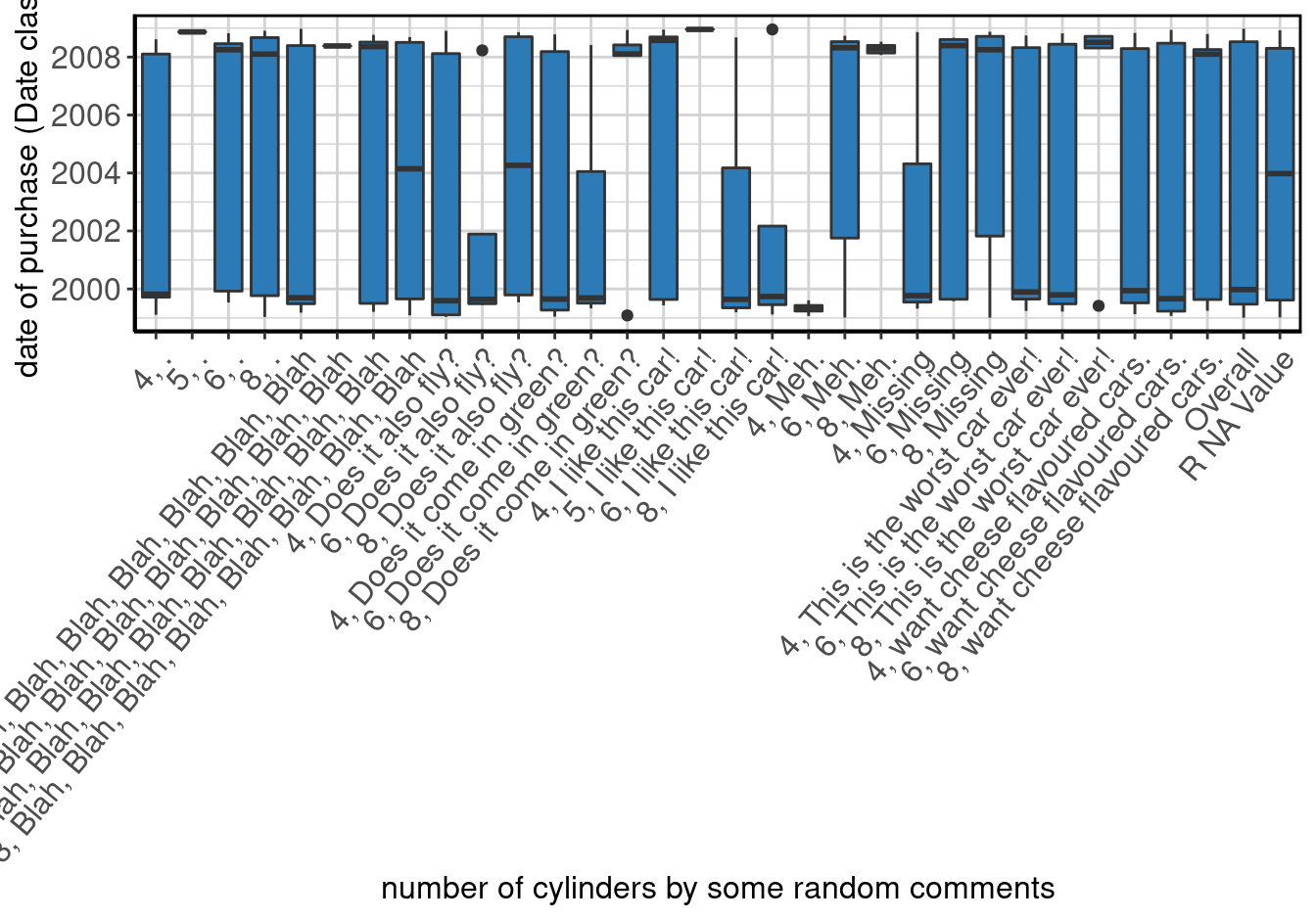
Figure 74: Boxplot of date of purchase (Date class) by number of cylinders by type of car.
Comments by Number of Cylinders by Class
The results are in table 94 and figure 75.
commentsByCylByClassSummary <- data_summary(x = "comments", by = c("cyl", "class"), data = mpg)

make_complete_output(commentsByCylByClassSummary)| some random comments | 4, 2seater | 5, 2seater | 6, 2seater | 8, 2seater | 4, compact | 5, compact | 6, compact | 8, compact | 4, midsize | 5, midsize | 6, midsize | 8, midsize | 4, minivan | 5, minivan | 6, minivan | 8, minivan | 4, pickup | 5, pickup | 6, pickup | 8, pickup | 4, subcompact | 5, subcompact | 6, subcompact | 8, subcompact | 4, suv | 5, suv | 6, suv | 8, suv | Overall |
|---|---|---|---|---|---|---|---|---|---|---|---|---|---|---|---|---|---|---|---|---|---|---|---|---|---|---|---|---|---|
| . | 0 (NaN%) | 0 (NaN%) | 0 (NaN%) | 1 (20%) | 2 (6.25%) | 0 (0%) | 1 (7.69%) | 0 (NaN%) | 1 (6.25%) | 0 (NaN%) | 4 (17.39%) | 0 (0%) | 0 (0%) | 0 (NaN%) | 1 (10%) | 0 (NaN%) | 0 (0%) | 0 (NaN%) | 1 (10%) | 4 (20%) | 1 (4.76%) | 1 (50%) | 1 (14.29%) | 1 (20%) | 1 (12.5%) | 0 (NaN%) | 1 (6.25%) | 5 (13.16%) | 26 (11.11%) |
| Blah, Blah, Blah, Blah, Blah, Blah, Blah, Blah | 0 (NaN%) | 0 (NaN%) | 0 (NaN%) | 0 (0%) | 3 (9.38%) | 2 (100%) | 0 (0%) | 0 (NaN%) | 3 (18.75%) | 0 (NaN%) | 3 (13.04%) | 0 (0%) | 0 (0%) | 0 (NaN%) | 0 (0%) | 0 (NaN%) | 1 (33.33%) | 0 (NaN%) | 2 (20%) | 1 (5%) | 0 (0%) | 0 (0%) | 2 (28.57%) | 1 (20%) | 2 (25%) | 0 (NaN%) | 1 (6.25%) | 2 (5.26%) | 23 (9.83%) |
| Does it also fly? | 0 (NaN%) | 0 (NaN%) | 0 (NaN%) | 0 (0%) | 1 (3.12%) | 0 (0%) | 0 (0%) | 0 (NaN%) | 1 (6.25%) | 0 (NaN%) | 4 (17.39%) | 1 (50%) | 0 (0%) | 0 (NaN%) | 1 (10%) | 0 (NaN%) | 0 (0%) | 0 (NaN%) | 0 (0%) | 0 (0%) | 3 (14.29%) | 0 (0%) | 0 (0%) | 0 (0%) | 0 (0%) | 0 (NaN%) | 2 (12.5%) | 3 (7.89%) | 16 (6.84%) |
| Does it come in green? | 0 (NaN%) | 0 (NaN%) | 0 (NaN%) | 0 (0%) | 7 (21.88%) | 0 (0%) | 1 (7.69%) | 0 (NaN%) | 3 (18.75%) | 0 (NaN%) | 0 (0%) | 0 (0%) | 0 (0%) | 0 (NaN%) | 0 (0%) | 0 (NaN%) | 0 (0%) | 0 (NaN%) | 0 (0%) | 0 (0%) | 3 (14.29%) | 0 (0%) | 0 (0%) | 0 (0%) | 2 (25%) | 0 (NaN%) | 2 (12.5%) | 5 (13.16%) | 23 (9.83%) |
| I like this car! | 0 (NaN%) | 0 (NaN%) | 0 (NaN%) | 0 (0%) | 4 (12.5%) | 0 (0%) | 3 (23.08%) | 0 (NaN%) | 3 (18.75%) | 0 (NaN%) | 1 (4.35%) | 0 (0%) | 0 (0%) | 0 (NaN%) | 1 (10%) | 0 (NaN%) | 1 (33.33%) | 0 (NaN%) | 2 (20%) | 2 (10%) | 2 (9.52%) | 1 (50%) | 0 (0%) | 0 (0%) | 0 (0%) | 0 (NaN%) | 2 (12.5%) | 2 (5.26%) | 24 (10.26%) |
| Meh. | 0 (NaN%) | 0 (NaN%) | 0 (NaN%) | 1 (20%) | 1 (3.12%) | 0 (0%) | 0 (0%) | 0 (NaN%) | 1 (6.25%) | 0 (NaN%) | 1 (4.35%) | 0 (0%) | 0 (0%) | 0 (NaN%) | 1 (10%) | 0 (NaN%) | 0 (0%) | 0 (NaN%) | 1 (10%) | 1 (5%) | 4 (19.05%) | 0 (0%) | 1 (14.29%) | 0 (0%) | 0 (0%) | 0 (NaN%) | 2 (12.5%) | 4 (10.53%) | 18 (7.69%) |
| Missing | 0 (NaN%) | 0 (NaN%) | 0 (NaN%) | 1 (20%) | 4 (12.5%) | 0 (0%) | 0 (0%) | 0 (NaN%) | 0 (0%) | 0 (NaN%) | 2 (8.7%) | 1 (50%) | 0 (0%) | 0 (NaN%) | 1 (10%) | 0 (NaN%) | 0 (0%) | 0 (NaN%) | 0 (0%) | 5 (25%) | 2 (9.52%) | 0 (0%) | 0 (0%) | 1 (20%) | 0 (0%) | 0 (NaN%) | 2 (12.5%) | 6 (15.79%) | 25 (10.68%) |
| This is the worst car ever! | 0 (NaN%) | 0 (NaN%) | 0 (NaN%) | 0 (0%) | 5 (15.62%) | 0 (0%) | 2 (15.38%) | 0 (NaN%) | 1 (6.25%) | 0 (NaN%) | 3 (13.04%) | 0 (0%) | 1 (100%) | 0 (NaN%) | 2 (20%) | 0 (NaN%) | 0 (0%) | 0 (NaN%) | 1 (10%) | 2 (10%) | 0 (0%) | 0 (0%) | 0 (0%) | 1 (20%) | 0 (0%) | 0 (NaN%) | 2 (12.5%) | 2 (5.26%) | 22 (9.4%) |
| want cheese flavoured cars. | 0 (NaN%) | 0 (NaN%) | 0 (NaN%) | 1 (20%) | 3 (9.38%) | 0 (0%) | 3 (23.08%) | 0 (NaN%) | 2 (12.5%) | 0 (NaN%) | 4 (17.39%) | 0 (0%) | 0 (0%) | 0 (NaN%) | 2 (20%) | 0 (NaN%) | 1 (33.33%) | 0 (NaN%) | 2 (20%) | 4 (20%) | 4 (19.05%) | 0 (0%) | 1 (14.29%) | 0 (0%) | 1 (12.5%) | 0 (NaN%) | 1 (6.25%) | 4 (10.53%) | 33 (14.1%) |
| R NA Value | 0 (NaN%) | 0 (NaN%) | 0 (NaN%) | 1 (20%) | 2 (6.25%) | 0 (0%) | 3 (23.08%) | 0 (NaN%) | 1 (6.25%) | 0 (NaN%) | 1 (4.35%) | 0 (0%) | 0 (0%) | 0 (NaN%) | 1 (10%) | 0 (NaN%) | 0 (0%) | 0 (NaN%) | 1 (10%) | 1 (5%) | 2 (9.52%) | 0 (0%) | 2 (28.57%) | 1 (20%) | 2 (25%) | 0 (NaN%) | 1 (6.25%) | 5 (13.16%) | 24 (10.26%) |
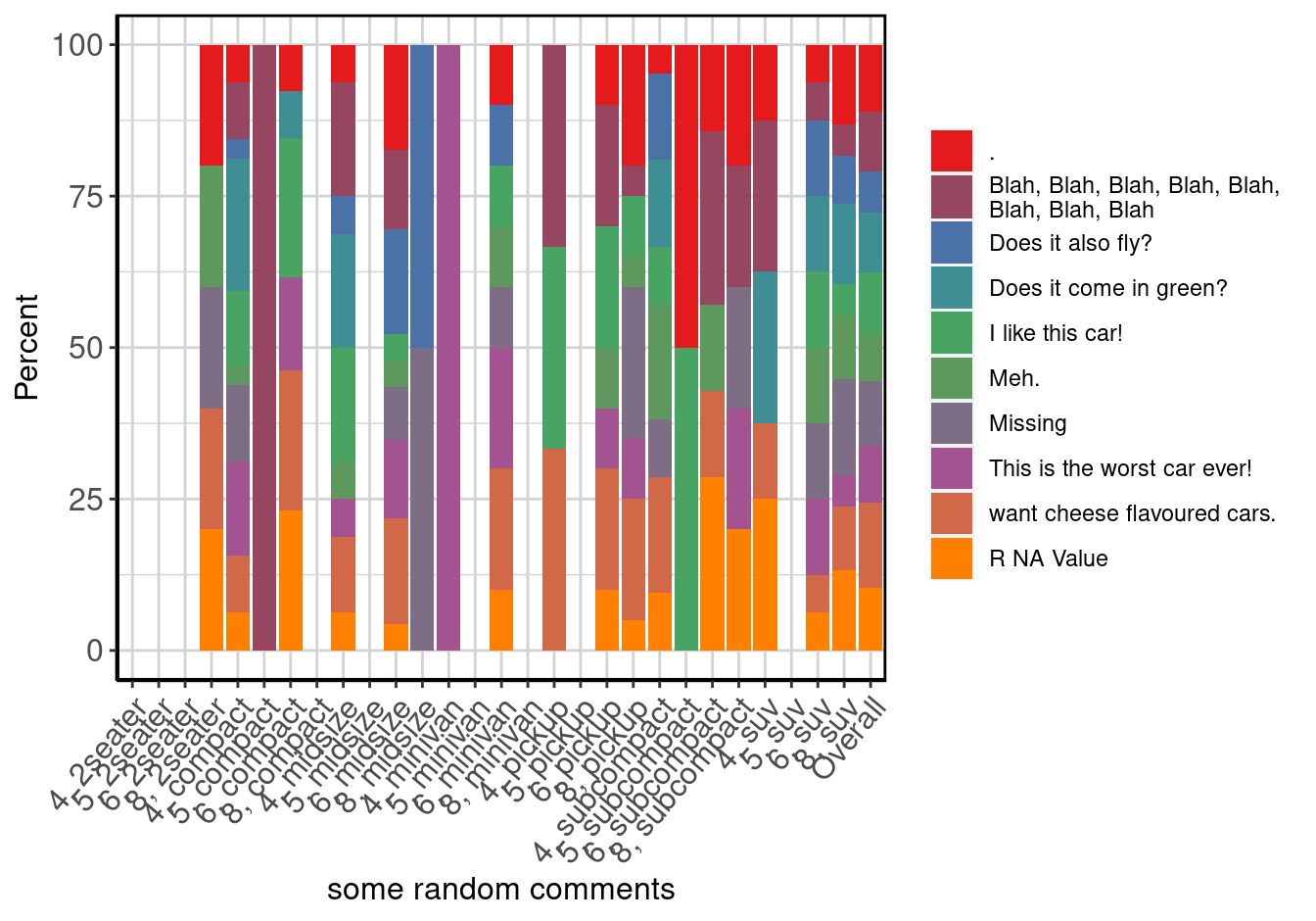
Figure 75: Stacked barplot of some random comments by number of cylinders by type of car.
Summary Tables
The full summaries with plots are useful for understanding the data and diagnosing issues, but eventually, you will want to summarise the data in a more digestible form.
Univariate Data Summaries
invisible(setGeneric(name = "univariate_data_summary", def = function(object) standardGeneric("univariate_data_summary")))
setMethod(f = "univariate_data_summary",
signature = "dataSummaries",
definition = function(object)
{
if(all(c("Mean", "S Dev") %in% colnames(object@table))) {
xlab <- paste("<b>", object@xLab, ", Mean (SD)</b>", sep = "")
if(length(object@difftime_units) > 0) {
res <- paste(object@table[, "Mean"], " (", object@table[, "S Dev"], " ", object@difftime_units, ")", sep = "")
} else {
res <- paste(object@table[, "Mean"], " (", object@table[, "S Dev"], ")", sep = "")
}
res <- data.frame(res)
res$rname <- xlab
res <- res[, c(2, 1)]
colnames(res) <- c("", "")
rownames(res) <- NULL
} else {
xlab <- paste("<b>", object@xLab, ", n (%)", "</b>", sep = "")
res <- c("", object@table[, -1])
res <- data.frame(res, stringsAsFactors = FALSE)
res$rnames <- c(xlab, paste(" ", as.character(object@table[, 1]), sep = ""))
res <- res[, c(2, 1)]
colnames(res) <- c("", "")
rownames(res) <- NULL
}
return(res)
}
)
univariateDataSummaryList <- list(
manuSummary,
modelSummary,
displSummary,
yearSummary,
dpSummary,
cylSummary,
transSummary,
drvSummary,
ctySummary,
hwySummary,
flSummary,
classSummary,
rnSummary,
rdifftimeSummary,
logicalSummary,
partySummary,
commentsSummary,
missSummary
)
cars_univariate_data_summary <- do.call("rbind", lapply(univariateDataSummaryList, univariate_data_summary))
kable(cars_univariate_data_summary, caption = "Data summaries", booktabs = TRUE, escape = FALSE) %>% kable_styling(bootstrap_options = c("striped", "hover", "condensed", "responsive"))| manufacturer, n (%) | |
| audi | 18 (7.69%) |
| chevrolet | 19 (8.12%) |
| dodge | 37 (15.81%) |
| ford | 25 (10.68%) |
| honda | 9 (3.85%) |
| hyundai | 14 (5.98%) |
| jeep | 8 (3.42%) |
| land rover | 4 (1.71%) |
| lincoln | 3 (1.28%) |
| mercury | 4 (1.71%) |
| nissan | 13 (5.56%) |
| pontiac | 5 (2.14%) |
| subaru | 14 (5.98%) |
| toyota | 34 (14.53%) |
| volkswagen | 27 (11.54%) |
| model name, n (%) | |
| 4runner 4wd | 6 (2.56%) |
| a4 | 7 (2.99%) |
| a4 quattro | 8 (3.42%) |
| a6 quattro | 3 (1.28%) |
| altima | 6 (2.56%) |
| c1500 suburban 2wd | 5 (2.14%) |
| camry | 7 (2.99%) |
| camry solara | 7 (2.99%) |
| caravan 2wd | 11 (4.7%) |
| civic | 9 (3.85%) |
| corolla | 5 (2.14%) |
| corvette | 5 (2.14%) |
| dakota pickup 4wd | 9 (3.85%) |
| durango 4wd | 7 (2.99%) |
| expedition 2wd | 3 (1.28%) |
| explorer 4wd | 6 (2.56%) |
| f150 pickup 4wd | 7 (2.99%) |
| forester awd | 6 (2.56%) |
| grand cherokee 4wd | 8 (3.42%) |
| grand prix | 5 (2.14%) |
| gti | 5 (2.14%) |
| impreza awd | 8 (3.42%) |
| jetta | 9 (3.85%) |
| k1500 tahoe 4wd | 4 (1.71%) |
| land cruiser wagon 4wd | 2 (0.85%) |
| malibu | 5 (2.14%) |
| maxima | 3 (1.28%) |
| mountaineer 4wd | 4 (1.71%) |
| mustang | 9 (3.85%) |
| navigator 2wd | 3 (1.28%) |
| new beetle | 6 (2.56%) |
| passat | 7 (2.99%) |
| pathfinder 4wd | 4 (1.71%) |
| ram 1500 pickup 4wd | 10 (4.27%) |
| range rover | 4 (1.71%) |
| sonata | 7 (2.99%) |
| tiburon | 7 (2.99%) |
| toyota tacoma 4wd | 7 (2.99%) |
| engine displacement, in litres, Mean (SD) | 3.47 (1.29) |
| year of manufacture, n (%) | |
| 1999 | 117 (50%) |
| 2008 | 117 (50%) |
| date of purchase (Date class), Mean (SD) | 2003-12-21 (236.59 weeks) |
| number of cylinders, n (%) | |
| 4 | 81 (34.62%) |
| 5 | 4 (1.71%) |
| 6 | 79 (33.76%) |
| 8 | 70 (29.91%) |
| type of transmission, n (%) | |
| auto(av) | 5 (2.14%) |
| auto(l3) | 2 (0.85%) |
| auto(l4) | 83 (35.47%) |
| auto(l5) | 39 (16.67%) |
| auto(l6) | 6 (2.56%) |
| auto(s4) | 3 (1.28%) |
| auto(s5) | 3 (1.28%) |
| auto(s6) | 16 (6.84%) |
| manual(m5) | 58 (24.79%) |
| manual(m6) | 19 (8.12%) |
| drive type, n (%) | |
| front-wheel drive | 106 (45.3%) |
| rear wheel drive | 25 (10.68%) |
| 4wd | 103 (44.02%) |
| city miles per gallon, Mean (SD) | 16.86 (4.26) |
| highway miles per gallon, Mean (SD) | 23.44 (5.95) |
| fuel type, n (%) | |
| c | 1 (0.43%) |
| d | 5 (2.14%) |
| e | 8 (3.42%) |
| p | 52 (22.22%) |
| r | 168 (71.79%) |
| type of car, n (%) | |
| 2seater | 5 (2.14%) |
| compact | 47 (20.09%) |
| midsize | 41 (17.52%) |
| minivan | 11 (4.7%) |
| pickup | 33 (14.1%) |
| subcompact | 35 (14.96%) |
| suv | 62 (26.5%) |
| some random numbers that are generated from a normal distrubtion with mean = 10 and sd = 5, Mean (SD) | 10.53 (5.09) |
| some random numbers that are generated from a normal distrubtion with mean = 10 and sd = 5, and then converted to weeks, Mean (SD) | 9.76 (5.07 weeks) |
| some random numbers that are generated from a normal distrubtion with mean = 10 and sd = 5, and then converted to weeks, and then set to TRUE if the difference is greater than 10, n (%) | |
| FALSE | 96 (41.03%) |
| TRUE | 88 (37.61%) |
| R NA Value | 50 (21.37%) |
| some random political parties, n (%) | |
| republican | 56 (23.93%) |
| democrat | 61 (26.07%) |
| independent | 62 (26.5%) |
| R NA Value | 55 (23.5%) |
| some random comments, n (%) | |
| . | 26 (11.11%) |
| Blah, Blah, Blah, Blah, Blah, Blah, Blah, Blah | 23 (9.83%) |
| Does it also fly? | 16 (6.84%) |
| Does it come in green? | 23 (9.83%) |
| I like this car! | 24 (10.26%) |
| Meh. | 18 (7.69%) |
| Missing | 25 (10.68%) |
| This is the worst car ever! | 22 (9.4%) |
| want cheese flavoured cars. | 33 (14.1%) |
| R NA Value | 24 (10.26%) |
| an all missing variable, n (%) | |
| R NA Value | 234 (100%) |
By Data Summaries
invisible(setGeneric(name = "by_data_summary", def = function(object) standardGeneric("by_data_summary")))
setMethod(f = "by_data_summary",
signature = "dataSummaries",
definition = function(object)
{
if(all(c("Mean", "S Dev") %in% colnames(object@table))) {
res <- t(object@table[, c("Mean", "S Dev")])
if(length(object@difftime_units) > 0) {
res <- paste(object@table[, "Mean"], " (", object@table[, "S Dev"], " ", object@difftime_units, ")", sep = "")
} else {
res <- paste(object@table[, "Mean"], " (", object@table[, "S Dev"], ")", sep = "")
}
res <- data.frame(t(res))
res$label <- paste("<b>", object@xLab, ", Mean (SD)</b>", sep = "")
rownames(res) <- NULL
res <- res[, c(which(colnames(res) == "label"), which(!(1:dim(res)[2] %in% which(colnames(res) == "label"))))]
colnames(res) <- c("", as.character(object@table[, 1]))
} else {
res <- object@table
res[, 1] <- paste(" ", res[, 1], sep = "")
res <- rbind("", res)
res[1,1] <- paste("<b>", object@xLab, ", N (%)</b>", sep = "")
colnames(res)[1] <- ""
}
return(res)
}
)
byDataSummaryList <- list(
ctyByDrvSummary,
hwyByDrvSummary,
cylByDrvSummary,
dpByDrvSummary,
rnByDrvSummary,
rdifftimeByDrvSummary,
logicalByDrvSummary,
commentsByDrvSummary,
missByDrvSummary
)
cars_by_data_summary <- do.call("rbind", lapply(byDataSummaryList, by_data_summary))
kable(cars_by_data_summary, caption = "Data summaries", booktabs = TRUE, escape = FALSE) %>% kable_styling(bootstrap_options = c("striped", "hover", "condensed", "responsive"))| front-wheel drive | rear wheel drive | 4wd | Overall | |
|---|---|---|---|---|
| city miles per gallon, Mean (SD) | 19.97 (3.63) | 14.08 (2.22) | 14.33 (2.87) | 16.86 (4.26) |
| highway miles per gallon, Mean (SD) | 28.16 (4.21) | 21 (3.66) | 19.17 (4.08) | 23.44 (5.95) |
| number of cylinders, N (%) | ||||
| 4 | 58 (54.72%) | 0 (0%) | 23 (22.33%) | 81 (34.62%) |
| 5 | 4 (3.77%) | 0 (0%) | 0 (0%) | 4 (1.71%) |
| 6 | 43 (40.57%) | 4 (16%) | 32 (31.07%) | 79 (33.76%) |
| 8 | 1 (0.94%) | 21 (84%) | 48 (46.6%) | 70 (29.91%) |
| date of purchase (Date class), Mean (SD) | 2003-06-08 (235.2 weeks) | 2004-09-28 (235.47 weeks) | 2004-04-21 (237.55 weeks) | 2003-12-21 (236.59 weeks) |
| some random numbers that are generated from a normal distrubtion with mean = 10 and sd = 5, Mean (SD) | 10.5 (5.32) | 11.59 (4.49) | 10.33 (4.99) | 10.53 (5.09) |
| some random numbers that are generated from a normal distrubtion with mean = 10 and sd = 5, and then converted to weeks, Mean (SD) | 10.57 (5.24 weeks) | 8.43 (5.17 weeks) | 9.19 (4.77 weeks) | 9.76 (5.07 weeks) |
| some random numbers that are generated from a normal distrubtion with mean = 10 and sd = 5, and then converted to weeks, and then set to TRUE if the difference is greater than 10, N (%) | ||||
| FALSE | 40 (37.74%) | 11 (44%) | 45 (43.69%) | 96 (41.03%) |
| TRUE | 46 (43.4%) | 8 (32%) | 34 (33.01%) | 88 (37.61%) |
| R NA Value | 20 (18.87%) | 6 (24%) | 24 (23.3%) | 50 (21.37%) |
| some random comments, N (%) | ||||
| . | 9 (8.49%) | 5 (20%) | 12 (11.65%) | 26 (11.11%) |
| Blah, Blah, Blah, Blah, Blah, Blah, Blah, Blah | 12 (11.32%) | 3 (12%) | 8 (7.77%) | 23 (9.83%) |
| Does it also fly? | 11 (10.38%) | 1 (4%) | 4 (3.88%) | 16 (6.84%) |
| Does it come in green? | 12 (11.32%) | 1 (4%) | 10 (9.71%) | 23 (9.83%) |
| I like this car! | 13 (12.26%) | 1 (4%) | 10 (9.71%) | 24 (10.26%) |
| Meh. | 6 (5.66%) | 2 (8%) | 10 (9.71%) | 18 (7.69%) |
| Missing | 8 (7.55%) | 3 (12%) | 14 (13.59%) | 25 (10.68%) |
| This is the worst car ever! | 14 (13.21%) | 2 (8%) | 6 (5.83%) | 22 (9.4%) |
| want cheese flavoured cars. | 13 (12.26%) | 2 (8%) | 18 (17.48%) | 33 (14.1%) |
| R NA Value | 8 (7.55%) | 5 (20%) | 11 (10.68%) | 24 (10.26%) |
| an all missing variable, N (%) | ||||
| R NA Value | 106 (100%) | 25 (100%) | 103 (100%) | 234 (100%) |
Bivariate Data Summaries
invisible(setGeneric(name = "bivariate_data_summary", def = function(object1, object2) standardGeneric("bivariate_data_summary")))
setMethod(f = "bivariate_data_summary",
signature = "dataSummaries",
definition = function(object1, object2)
{
rnames <- c(paste("<b>", object1@byLab, "</b>", sep = ""), paste(" ", object1@table[, 1], sep = ""))
if(length(object1@difftime_units) > 0) {
object1Res <- data.frame(c("", paste(object1@table[, "Mean"], " (", object1@table[, "S Dev"], " ", object1@difftime_units, ")", sep = "")), stringsAsFactors = FALSE)
} else {
object1Res <- data.frame(c("", paste(object1@table[, "Mean"], " (", object1@table[, "S Dev"], ")", sep = "")), stringsAsFactors = FALSE)
}
if(length(object2@difftime_units) > 0) {
object2Res <- data.frame(c("", paste(object2@table[, "Mean"], " (", object1@table[, "S Dev"], " ", object2@difftime_units, ")", sep = "")), stringsAsFactors = FALSE)
} else {
object2Res <- data.frame(c("", paste(object2@table[, "Mean"], " (", object2@table[, "S Dev"], ")", sep = "")), stringsAsFactors = FALSE)
}
res <- cbind(object1Res, object2Res)
res <- cbind(rnames, res)
colnames(res) <- c("", paste(object1@xLab, ", Mean (SD)", sep = ""), paste(object2@xLab, ", Mean (SD)", sep = ""))
return(res)
}
)
cars_bivariate_data_summary <- rbind(
bivariate_data_summary(ctyBymanuSummary, hwyBymanuSummary),
bivariate_data_summary(ctyBymodelSummary, hwyBymodelSummary),
bivariate_data_summary(ctyByYearSummary, hwyByYearSummary),
bivariate_data_summary(ctyByCylSummary, hwyByCylSummary),
bivariate_data_summary(ctyBytransSummary, hwyBytransSummary),
bivariate_data_summary(ctyByDrvSummary, hwyByDrvSummary),
bivariate_data_summary(ctyByflSummary, hwyByflSummary),
bivariate_data_summary(ctyByclassSummary, hwyByclassSummary),
bivariate_data_summary(ctyByPartySummary, hwyByPartySummary),
bivariate_data_summary(ctyByCommentsSummary, hwyByCommentsSummary),
bivariate_data_summary(ctyByMissSummary, hwyByMissSummary)
)
kable(cars_bivariate_data_summary, caption = "By data summaries of miles per gallons for city and highway.", booktabs = TRUE, escape = FALSE) %>% kable_styling(bootstrap_options = c("striped", "hover", "condensed", "responsive"))| city miles per gallon, Mean (SD) | highway miles per gallon, Mean (SD) | |
|---|---|---|
| manufacturer | ||
| audi | 17.61 (1.97) | 26.44 (2.18) |
| chevrolet | 15 (2.92) | 21.89 (5.11) |
| dodge | 13.14 (2.49) | 17.95 (3.57) |
| ford | 14 (1.91) | 19.36 (3.33) |
| honda | 24.44 (1.94) | 32.56 (2.55) |
| hyundai | 18.64 (1.5) | 26.86 (2.18) |
| jeep | 13.5 (2.51) | 17.62 (3.25) |
| land rover | 11.5 (0.58) | 16.5 (1.73) |
| lincoln | 11.33 (0.58) | 17 (1) |
| mercury | 13.25 (0.5) | 18 (1.15) |
| nissan | 18.08 (3.43) | 24.62 (5.09) |
| pontiac | 17 (1) | 26.4 (1.14) |
| subaru | 19.29 (0.91) | 25.57 (1.16) |
| toyota | 18.53 (4.05) | 24.91 (6.17) |
| volkswagen | 20.93 (4.56) | 29.22 (5.32) |
| Overall | 16.86 (4.26) | 23.44 (5.95) |
| model name | ||
| 4runner 4wd | 15.17 (0.75) | 18.83 (1.47) |
| a4 | 18.86 (1.86) | 28.29 (1.98) |
| a4 quattro | 17.12 (1.81) | 25.75 (1.16) |
| a6 quattro | 16 (1) | 24 (1) |
| altima | 20.67 (1.97) | 28.67 (2.42) |
| c1500 suburban 2wd | 12.8 (1.3) | 17.8 (2.17) |
| camry | 19.86 (1.46) | 28.29 (2.14) |
| camry solara | 19.86 (1.77) | 28.14 (2.19) |
| caravan 2wd | 15.82 (1.83) | 22.36 (2.06) |
| civic | 24.44 (1.94) | 32.56 (2.55) |
| corolla | 25.6 (1.67) | 34 (2.65) |
| corvette | 15.4 (0.55) | 24.8 (1.3) |
| dakota pickup 4wd | 12.78 (1.99) | 17 (2.29) |
| durango 4wd | 11.86 (1.57) | 16 (2) |
| expedition 2wd | 11.33 (0.58) | 17.33 (0.58) |
| explorer 4wd | 13.67 (0.82) | 18 (1.1) |
| f150 pickup 4wd | 13 (1) | 16.43 (0.79) |
| forester awd | 18.83 (0.98) | 25 (1.41) |
| grand cherokee 4wd | 13.5 (2.51) | 17.62 (3.25) |
| grand prix | 17 (1) | 26.4 (1.14) |
| gti | 20 (2) | 27.4 (2.3) |
| impreza awd | 19.62 (0.74) | 26 (0.76) |
| jetta | 21.22 (4.87) | 29.11 (6.07) |
| k1500 tahoe 4wd | 12.5 (1.73) | 16.25 (2.22) |
| land cruiser wagon 4wd | 12 (1.41) | 16.5 (2.12) |
| malibu | 18.8 (1.92) | 27.6 (1.82) |
| maxima | 18.67 (0.58) | 25.33 (0.58) |
| mountaineer 4wd | 13.25 (0.5) | 18 (1.15) |
| mustang | 15.89 (1.45) | 23.22 (2.17) |
| navigator 2wd | 11.33 (0.58) | 17 (1) |
| new beetle | 24 (6.51) | 32.83 (7.63) |
| passat | 18.57 (1.9) | 27.57 (1.51) |
| pathfinder 4wd | 13.75 (1.26) | 18 (1.41) |
| ram 1500 pickup 4wd | 11.4 (1.51) | 15.3 (1.89) |
| range rover | 11.5 (0.58) | 16.5 (1.73) |
| sonata | 19 (1.41) | 27.71 (2.06) |
| tiburon | 18.29 (1.6) | 26 (2.08) |
| toyota tacoma 4wd | 15.57 (0.79) | 19.43 (1.62) |
| Overall | 16.86 (4.26) | 23.44 (5.95) |
| year of manufacture | ||
| 1999 | 17.02 (4.46) | 23.43 (6.08) |
| 2008 | 16.7 (4.06) | 23.45 (5.85) |
| Overall | 16.86 (4.26) | 23.44 (5.95) |
| number of cylinders | ||
| 4 | 21.01 (3.5) | 28.8 (4.52) |
| 5 | 20.5 (0.58) | 28.75 (0.5) |
| 6 | 16.22 (1.77) | 22.82 (3.69) |
| 8 | 12.57 (1.81) | 17.63 (3.26) |
| Overall | 16.86 (4.26) | 23.44 (5.95) |
| type of transmission | ||
| auto(av) | 20 (2) | 27.8 (2.59) |
| auto(l3) | 21 (4.24) | 27 (4.24) |
| auto(l4) | 15.94 (3.98) | 21.96 (5.64) |
| auto(l5) | 14.72 (3.49) | 20.72 (6.04) |
| auto(l6) | 13.67 (1.86) | 20 (2.37) |
| auto(s4) | 18.67 (2.31) | 25.67 (1.15) |
| auto(s5) | 17.33 (5.03) | 25.33 (6.66) |
| auto(s6) | 17.38 (3.22) | 25.19 (3.99) |
| manual(m5) | 19.26 (4.56) | 26.29 (5.99) |
| manual(m6) | 16.89 (3.83) | 24.21 (5.75) |
| Overall | 16.86 (4.26) | 23.44 (5.95) |
| drive type | ||
| front-wheel drive | 19.97 (3.63) | 28.16 (4.21) |
| rear wheel drive | 14.08 (2.22) | 21 (3.66) |
| 4wd | 14.33 (2.87) | 19.17 (4.08) |
| Overall | 16.86 (4.26) | 23.44 (5.95) |
| fuel type | ||
| c | 24 (NA) | 36 (NA) |
| d | 25.6 (9.53) | 33.6 (13.05) |
| e | 9.75 (1.04) | 13.25 (1.91) |
| p | 17.37 (3.04) | 25.23 (3.93) |
| r | 16.74 (3.89) | 22.99 (5.51) |
| Overall | 16.86 (4.26) | 23.44 (5.95) |
| type of car | ||
| 2seater | 15.4 (0.55) | 24.8 (1.3) |
| compact | 20.13 (3.39) | 28.3 (3.78) |
| midsize | 18.76 (1.95) | 27.29 (2.14) |
| minivan | 15.82 (1.83) | 22.36 (2.06) |
| pickup | 13 (2.05) | 16.88 (2.27) |
| subcompact | 20.37 (4.6) | 28.14 (5.38) |
| suv | 13.5 (2.42) | 18.13 (2.98) |
| Overall | 16.86 (4.26) | 23.44 (5.95) |
| some random political parties | ||
| republican | 17.29 (4.52) | 23.57 (6.42) |
| democrat | 16.26 (4.59) | 22.38 (6.25) |
| independent | 16.84 (3.39) | 23.68 (4.83) |
| Overall | 16.86 (4.26) | 23.44 (5.95) |
| R NA Value | 17.11 (4.5) | 24.22 (6.26) |
| some random comments | ||
| . | 15.42 (3.94) | 22.08 (5.6) |
| Blah, Blah, Blah, Blah, Blah, Blah, Blah, Blah | 17.04 (3.23) | 24.09 (4.95) |
| Does it also fly? | 17.94 (5.52) | 24.75 (7.33) |
| Does it come in green? | 18.39 (4.31) | 25.26 (5.5) |
| I like this car! | 17.92 (5.16) | 24.75 (7.25) |
| Meh. | 16.33 (3.4) | 22.61 (4.58) |
| Missing | 15.84 (5.16) | 21.96 (7.33) |
| This is the worst car ever! | 17.09 (4) | 23.82 (5.78) |
| want cheese flavoured cars. | 16.91 (3.95) | 23.33 (5.85) |
| Overall | 16.86 (4.26) | 23.44 (5.95) |
| R NA Value | 16.17 (3.34) | 22.33 (4.72) |
| an all missing variable | ||
| Overall | 16.86 (4.26) | 23.44 (5.95) |
| R NA Value | 16.86 (4.26) | 23.44 (5.95) |
cars_bivariate_time_data_summary <- rbind(
  bivariate_data_summary(ctyByPartySummary, rdifftimeByPartySummary),
  bivariate_data_summary(ctyByCommentsSummary, rdifftimeByCommentsSummary)
)

kable(cars_bivariate_time_data_summary, caption = "By data summaries of miles per gallons for city and random difference in time.", booktabs = TRUE, escape = FALSE) %>% kable_styling(bootstrap_options = c("striped", "hover", "condensed", "responsive"))| city miles per gallon, Mean (SD) | some random numbers that are generated from a normal distrubtion with mean = 10 and sd = 5, and then converted to weeks, Mean (SD) | |
|---|---|---|
| some random political parties | ||
| republican | 17.29 (4.52) | 9.5 (4.52 weeks) |
| democrat | 16.26 (4.59) | 9.31 (4.59 weeks) |
| independent | 16.84 (3.39) | 10.22 (3.39 weeks) |
| Overall | 16.86 (4.26) | 9.76 (4.26 weeks) |
| R NA Value | 17.11 (4.5) | 10.08 (4.5 weeks) |
| some random comments | ||
| . | 15.42 (3.94) | 8.21 (3.94 weeks) |
| Blah, Blah, Blah, Blah, Blah, Blah, Blah, Blah | 17.04 (3.23) | 8.32 (3.23 weeks) |
| Does it also fly? | 17.94 (5.52) | 9.49 (5.52 weeks) |
| Does it come in green? | 18.39 (4.31) | 8.51 (4.31 weeks) |
| I like this car! | 17.92 (5.16) | 10.44 (5.16 weeks) |
| Meh. | 16.33 (3.4) | 10.21 (3.4 weeks) |
| Missing | 15.84 (5.16) | 11.44 (5.16 weeks) |
| This is the worst car ever! | 17.09 (4) | 9.28 (4 weeks) |
| want cheese flavoured cars. | 16.91 (3.95) | 10.88 (3.95 weeks) |
| Overall | 16.86 (4.26) | 9.76 (4.26 weeks) |
| R NA Value | 16.17 (3.34) | 10.69 (3.34 weeks) |
Session Info
sessionInfo()## R version 4.1.1 (2021-08-10)
## Platform: x86_64-pc-linux-gnu (64-bit)
## Running under: Ubuntu 20.04.3 LTS
##
## Matrix products: default
## BLAS: /usr/lib/x86_64-linux-gnu/blas/libblas.so.3.9.0
## LAPACK: /usr/lib/x86_64-linux-gnu/lapack/liblapack.so.3.9.0
##
## locale:
## [1] LC_CTYPE=C.UTF-8 LC_NUMERIC=C LC_TIME=C.UTF-8
## [4] LC_COLLATE=C.UTF-8 LC_MONETARY=C.UTF-8 LC_MESSAGES=C.UTF-8
## [7] LC_PAPER=C.UTF-8 LC_NAME=C LC_ADDRESS=C
## [10] LC_TELEPHONE=C LC_MEASUREMENT=C.UTF-8 LC_IDENTIFICATION=C
##
## attached base packages:
## [1] stats graphics grDevices datasets utils methods base
##
## other attached packages:
## [1] dplyr_1.0.7 reshape2_1.4.4 Hmisc_4.5-0 Formula_1.2-4
## [5] survival_3.2-12 lattice_0.20-44 ggplot2_3.3.5 kableExtra_1.3.4
## [9] bookdown_0.24 knitr_1.34
##
## loaded via a namespace (and not attached):
## [1] Rcpp_1.0.7 svglite_2.0.0 png_0.1-7
## [4] digest_0.6.27 utf8_1.2.2 plyr_1.8.6
## [7] R6_2.5.1 backports_1.2.1 evaluate_0.14
## [10] highr_0.9 httr_1.4.2 pillar_1.6.2
## [13] rlang_0.4.11 rstudioapi_0.13 data.table_1.14.0
## [16] jquerylib_0.1.4 rpart_4.1-15 Matrix_1.3-4
## [19] checkmate_2.0.0 rmarkdown_2.11 labeling_0.4.2
## [22] splines_4.1.1 webshot_0.5.2 stringr_1.4.0
## [25] foreign_0.8-81 htmlwidgets_1.5.4 munsell_0.5.0
## [28] compiler_4.1.1 xfun_0.26 pkgconfig_2.0.3
## [31] systemfonts_1.0.2 base64enc_0.1-3 htmltools_0.5.2
## [34] nnet_7.3-16 tidyselect_1.1.1 tibble_3.1.4
## [37] gridExtra_2.3 htmlTable_2.2.1 fansi_0.5.0
## [40] viridisLite_0.4.0 crayon_1.4.1 withr_2.4.2
## [43] grid_4.1.1 gtable_0.3.0 lifecycle_1.0.0
## [46] magrittr_2.0.1 scales_1.1.1 stringi_1.7.4
## [49] farver_2.1.0 renv_0.12.2 latticeExtra_0.6-29
## [52] xml2_1.3.2 ellipsis_0.3.2 generics_0.1.0
## [55] vctrs_0.3.8 RColorBrewer_1.1-2 tools_4.1.1
## [58] glue_1.4.2 purrr_0.3.4 jpeg_0.1-9
## [61] fastmap_1.1.0 yaml_2.2.1 colorspace_2.0-2
## [64] cluster_2.1.2 rvest_1.0.1
Comments
The results are in table 54 and figure 35.
Figure 35: Stacked barplot of some random comments.