Introduction

The general linear model (GLM), more commonly called linear regression, is the most common statistical modeling tool a statistician or data scientist will use. As such, it is crucial to know how to present results from a GLM in a way that is understandable to your audience.

The GLM assumes that the conditional distribution of the \(i^{th}\) response is normal with expectation that is a linear function of a set of \(p\) predictors with uncorrelated errors that represent the aggregate omitted causes of Y (equation (1)) (Fox 2008).

\[\begin{equation} Y_{i} \sim N(\beta_0 + X_{i1}\beta_{1} + + X_{i2}\beta_{2} + ... + X_{ip}\beta_{p}, \sigma_{\epsilon}^2) \tag{1} \end{equation}\]

This presentation uses the R programming language and assumes the end user is taking advantage of RStudio IDE to compile their R markdown files into HTML (R Core Team 2019; RStudio Team 2016). All of the files needed to reproduce these results can be downloaded from the Git repository git clone https://git.waderstats.com/regression_output/.

Required Libraries

The libraries knitr, bookdown, and kableExtra are used to generate the HTML output (Xie 2019, 2018; Zhu 2019). The ggplot2 library is loaded for the example data set that is used in this presentation (Wickham 2016). The Hmisc library provides functionality needed to create variable labels (Harrell Jr, Charles Dupont, and others. 2019). Regression diagnostics are plotted using the ggfortify package (Tang, Horikoshi, and Li 2016). The stargazer library will be used create nice looking regression output (Hlavac 2018).

package_loader <- function(x, ...) {
  if (x %in% rownames(installed.packages()) == FALSE) install.packages(x)
  library(x, ...)
}

packages <- c("knitr", "bookdown", "kableExtra", "ggplot2", "Hmisc", "ggfortify", "stargazer")

invisible(sapply(X = packages, FUN = package_loader, character.only = TRUE))

Example Data Setup

The data set used in this presentation is mpg from the ggplot2 package. From the description in the manual:

This dataset contains a subset of the fuel economy data that the EPA makes available here. It contains only models which had a new release every year between 1999 and 2008 - this was used as a proxy for the popularity of the car.

set.seed(123)
data(mpg)
mpg <- data.frame(mpg)

colnames(mpg)[which(colnames(mpg) == "manufacturer")] <- "manu"

mpg$manu <- factor(mpg$manu)
mpg$model <- factor(mpg$model)
mpg$displ <- as.numeric(mpg$displ)
mpg$year <- factor(mpg$year, levels = c("1999", "2008"), ordered = TRUE)

mpg$dp <- as.Date(NA, origin = "1970-01-01")
mpg$dp[which(mpg$year == "1999")] <- sample(seq(as.Date('1999-01-01', format = "%Y-%m-%d", origin = "1970-01-01"), as.Date('1999-12-25', format = "%Y-%m-%d", origin = "1970-01-01"), by="day"), dim(mpg)[1]/2)
mpg$dp[which(mpg$year == "2008")] <- sample(seq(as.Date('2008-01-01', format = "%Y-%m-%d", origin = "1970-01-01"), as.Date('2008-12-25', format = "%Y-%m-%d", origin = "1970-01-01"), by="day"), dim(mpg)[1]/2)

mpg$cyl <- factor(mpg$cyl, levels = c(4, 5, 6, 8), ordered = TRUE)
mpg$trans <- factor(mpg$trans)
mpg$drv <- factor(mpg$drv, levels = c("f", "r", "4"), labels = c("front-wheel drive", "rear wheel drive", "4wd"))
mpg$fl <- factor(mpg$fl)
mpg$class <- factor(mpg$class)

mpg$rn <- rnorm(dim(mpg)[1], mean = 10, sd = 5)
mpg$rn[sample(1:length(mpg$rn), size = 50)] <- NA

mpg$party <- factor(sample(c("republican", "democrat", "independent", NA), dim(mpg)[1], replace = TRUE), levels = c("republican", "democrat", "independent"))
mpg$comments <- sample(c("I like this car!", "Meh.", "This is the worst car ever!", "Does it come in green?", "want cheese flavoured cars.", "Does it also fly?", "Blah, Blah, Blah, Blah, Blah, Blah, Blah, Blah", NA), dim(mpg)[1], replace = TRUE)

label(mpg$manu) <- "manufacturer"
label(mpg$model) <- "model name"
label(mpg$displ) <- "engine displacement, in litres"
label(mpg$year) <- "year of manufacture"
label(mpg$dp) <- "date of purchase"
label(mpg$cyl) <- "number of cylinders"
label(mpg$trans) <- "type of transmission"
label(mpg$drv) <- "drive type"
label(mpg$cty) <- "city miles per gallon"
label(mpg$hwy) <- "highway miles per gallon"
label(mpg$fl) <- "fuel type"
label(mpg$class) <- "type of car"
label(mpg$rn) <- "some random numbers that are generated from a normal distrubtion with mean = 10 and sd = 5"
label(mpg$party) <- "some random political parties"
label(mpg$comments) <- "some random comments"

kable(head(mpg), caption = "Header of <b>mpg</b>.", booktabs = TRUE, escape = FALSE) %>% kable_styling(bootstrap_options = c("striped", "hover", "condensed", "responsive"))

Table 1: Header of **mpg**.
manu	model	displ	year	cyl	trans	drv	cty	hwy	fl	class	dp	rn	party	comments
audi	a4	1.8	1999	4	auto(l5)	front-wheel drive	18	29	p	compact	1999-06-28	18.98570	democrat	I like this car!
audi	a4	1.8	1999	4	manual(m5)	front-wheel drive	21	29	p	compact	1999-01-14	NA	NA	I like this car!
audi	a4	2.0	2008	4	manual(m6)	front-wheel drive	20	31	p	compact	2008-02-08	19.50450	independent	Does it also fly?
audi	a4	2.0	2008	4	auto(av)	front-wheel drive	21	30	p	compact	2008-07-14	NA	independent	I like this car!
audi	a4	2.8	1999	6	auto(l5)	front-wheel drive	16	26	p	compact	1999-07-14	13.68097	democrat	Meh.
audi	a4	2.8	1999	6	manual(m5)	front-wheel drive	18	26	p	compact	1999-11-02	16.82888	NA	Meh.

City MPG Regression

Model building starts with what predictors we hypothesize that the outcome depends on. In this case, I hypothesize that miles per gallon in the city and highway depends on a constant, engine displacement, year of manufacture, the number of cylinders, drive type, fuel type, and type of car, some random numbers, and political party affiliation (equations (2) and (3)).

\[\begin{equation} cty_{i} = \beta_0 + dipl_{i}\beta_{1} + year_{i}\beta_{2} + cyl_{i}\beta_{3} + drv_{i}\beta_{4} + \\class_{i}\beta_{5} + rn_{i}\beta_{6} + party_{i}\beta_{7} + \epsilon_{i} \tag{2} \end{equation}\]

\[\begin{equation} hwy_{i} = \beta_0 + dipl_{i}\beta_{1} + year_{i}\beta_{2} + cyl_{i}\beta_{3} + drv_{i}\beta_{4} + \\class_{i}\beta_{5} + rn_{i}\beta_{6} + party_{i}\beta_{7} + \epsilon_{i} \tag{3} \end{equation}\]

Regression Diagnostics

The regression diagnostics show a few problems. The residuals vs. fitted plot shows a few points that have large residuals. These points translate to a normal quantile plot with a large discrepancy between the standardized residuals and the theoretical quantiles on the tail. From the scale location plots, we see relative homoscedasticity except for the outliers. The plot of Cook’s distance, a measure of influence on the fit, shows that the outliers have a disproportionate influence on the estimates in the final fit.

ctyFit <- lm(cty ~ displ + year + cyl + drv + class + rn + party, data = mpg)

autoplot(ctyFit, which = c(1, 2, 3, 4), ncol = 2, label.size = 3)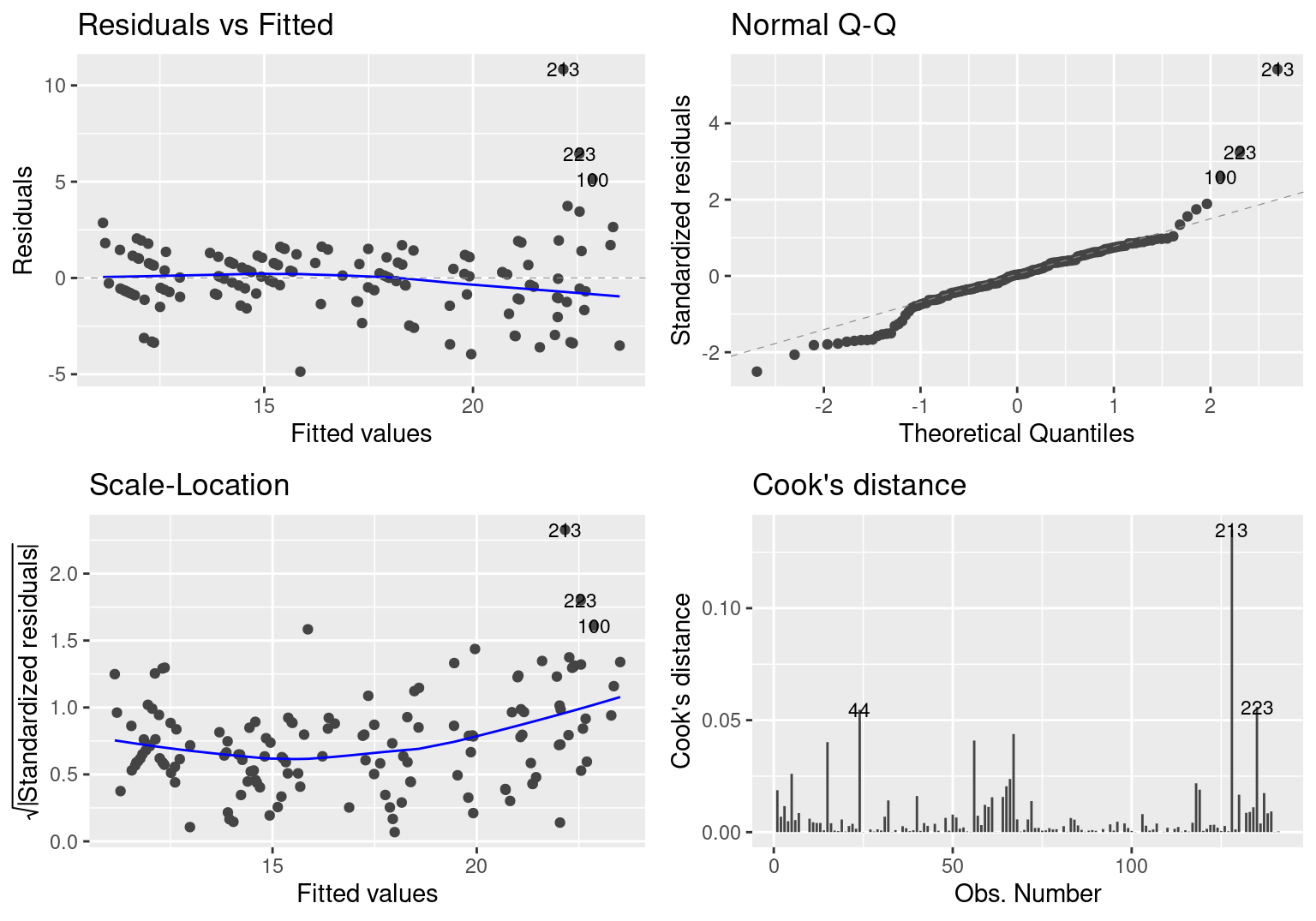

Figure 1: City MPG Regression Diagnostics

hwyFit <- lm(hwy ~ displ + year + cyl + drv + class + rn + party, data = mpg)

autoplot(hwyFit, which = c(1, 2, 3, 4), ncol = 2, label.size = 3)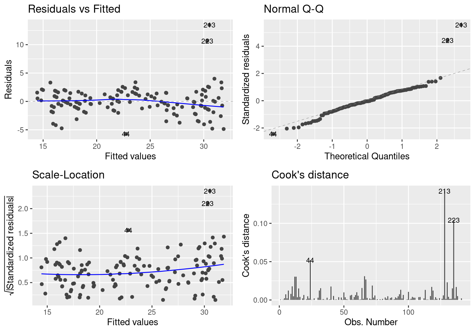

Figure 2: Highway MPG Regression Diagnostics

Regression Output

The regression starts with re-fitting the models with the problem points removed. Finally, we use the stargazer function to print the results. To customzie the disply the results, we also need a bit of css which can be downloaded here. The id for the CSS is generated by adding {#regression} to the header of this section. Check the markdown to see it in context.

ctyFit <- lm(cty ~ displ + year + cyl + drv + class + rn + party, data = mpg[c(-213, -223), ])

hwyFit <- lm(hwy ~ displ + year + cyl + drv + class + rn + party, data = mpg[c(-213, -223), ])

depLabels <- c(label(mpg$cty), label(mpg$hwy))

indepLabels <- c(
  "intercept",
  label(mpg$displ), 
  paste(label(mpg$year), ": ", levels(mpg$year)[2], " (ref = ", levels(mpg$year)[1], ")", sep = ""),
  paste(label(mpg$cyl), ": ", levels(mpg$cyl)[2], " (ref = ", levels(mpg$cyl)[1], ")", sep = ""),
  paste(label(mpg$cyl), ": ", levels(mpg$cyl)[3], " (ref = ", levels(mpg$cyl)[1], ")", sep = ""),
  paste(label(mpg$cyl), ": ", levels(mpg$cyl)[4], " (ref = ", levels(mpg$cyl)[1], ")", sep = ""),
  paste(label(mpg$drv), ": ", levels(mpg$drv)[2], " (ref = ", levels(mpg$drv)[1], ")", sep = ""), 
  paste(label(mpg$drv), ": ", levels(mpg$drv)[3], " (ref = ", levels(mpg$drv)[1], ")", sep = ""), 
  paste(label(mpg$class), ": ", levels(mpg$class)[2], " (ref = ", levels(mpg$class)[1], ")", sep = ""), 
  paste(label(mpg$class), ": ", levels(mpg$class)[3], " (ref = ", levels(mpg$class)[1], ")", sep = ""), 
  paste(label(mpg$class), ": ", levels(mpg$class)[4], " (ref = ", levels(mpg$class)[1], ")", sep = ""), 
  paste(label(mpg$class), ": ", levels(mpg$class)[5], " (ref = ", levels(mpg$class)[1], ")", sep = ""), 
  paste(label(mpg$class), ": ", levels(mpg$class)[6], " (ref = ", levels(mpg$class)[1], ")", sep = ""), 
  paste(label(mpg$class), ": ", levels(mpg$class)[7], " (ref = ", levels(mpg$class)[1], ")", sep = ""), 
  label(mpg$rn),
  paste(label(mpg$party), ": ", levels(mpg$party)[2], " (ref = ", levels(mpg$party)[1], ")", sep = ""),
  paste(label(mpg$party), ": ", levels(mpg$party)[3], " (ref = ", levels(mpg$party)[1], ")", sep = "")
)

stargazer(ctyFit, hwyFit, type = "html",
          title="Regression Results", 
          dep.var.labels = depLabels,
          covariate.labels = indepLabels,
          ci = TRUE,
          ci.level = 0.95,
          single.row = TRUE,
          align = TRUE,
          intercept.bottom = FALSE,
          intercept.top = TRUE
)

**Regression Results**

	Dependent variable:

	city miles per gallon	highway miles per gallon
	(1)	(2)

intercept	22.750^*** (18.368, 27.132)	33.366^*** (28.412, 38.320)
engine displacement, in litres	-0.382 (-1.231, 0.466)	-0.648 (-1.607, 0.311)
year of manufacture: 2008 (ref = 1999)	0.601^*** (0.167, 1.035)	0.991^*** (0.501, 1.482)
number of cylinders: 5 (ref = 4)	-3.414^*** (-5.096, -1.731)	-3.302^*** (-5.204, -1.400)
number of cylinders: 6 (ref = 4)	-0.173 (-1.277, 0.930)	-0.162 (-1.409, 1.085)
number of cylinders: 8 (ref = 4)	-0.408 (-1.773, 0.957)	-0.469 (-2.012, 1.074)
drive type: rear wheel drive (ref = front-wheel drive)	-1.964^** (-3.541, -0.387)	-1.585^* (-3.368, 0.197)
drive type: 4wd (ref = front-wheel drive)	-2.141^*** (-3.285, -0.996)	-2.844^*** (-4.138, -1.551)
type of car: compact (ref = 2seater)	-2.217 (-5.161, 0.727)	-3.440^** (-6.768, -0.112)
type of car: midsize (ref = 2seater)	-2.712^* (-5.704, 0.281)	-3.874^** (-7.257, -0.491)
type of car: minivan (ref = 2seater)	-4.975^*** (-8.102, -1.847)	-7.913^*** (-11.448, -4.378)
type of car: pickup (ref = 2seater)	-4.025^*** (-6.911, -1.138)	-8.987^*** (-12.250, -5.724)
type of car: subcompact (ref = 2seater)	-1.453 (-4.320, 1.414)	-3.592^** (-6.833, -0.351)
type of car: suv (ref = 2seater)	-3.673^*** (-6.397, -0.950)	-7.731^*** (-10.810, -4.653)
some random numbers that are generated from a normal distrubtion with mean = 10 and sd = 5	-0.039 (-0.092, 0.015)	-0.053^* (-0.113, 0.008)
some random political parties: democrat (ref = republican)	-0.169 (-0.973, 0.634)	-0.517 (-1.425, 0.392)
some random political parties: independent (ref = republican)	-0.175 (-0.937, 0.587)	-0.298 (-1.160, 0.563)

Observations	139	139
R²	0.830	0.891
Adjusted R²	0.807	0.876
Residual Std. Error (df = 122)	1.722	1.946
F Statistic (df = 16; 122)	37.128^***	62.027^***

Note:	p<0.1; p<0.05; p<0.01

Regression Summary

Using copy and paste to summarize results leaves a ton of room to make errors. To prevent this, we can summarize the results using inline R code. Check out the markdown file for how I did it in this case.

ctyCoef <- coef(ctyFit)
ctyConf <- confint(ctyFit)
ctyRes <- cbind(ctyCoef, ctyConf)

hwyCoef <- coef(hwyFit)
hwyConf <- confint(hwyFit)
hwyRes <- cbind(hwyCoef, hwyConf)

inlineReg <- function(x, lab) {
  r1 <- round(x[lab, 1], 1)
  r2 <- round(x[lab, 2], 1)
  r3 <- round(x[lab, 3], 1)

  res <- paste(r1, " (95% CI = [", r2, ",", r3, "])", sep = "")
  
  return(res)
}

The results show that highway MPG is much better than city MPG, with 22.7 (95% CI = [18.3,27.2]) and 33.4 (95% CI = [28.4,38.4]) respectively. We found that as compared to 1999, cars built in 2008 had an increase of 0.6 (95% CI = [0.2,1]) in city MPG and 1 (95% CI = [0.5,1.5]) in highway MPG. We found that minivans have the worst MPG as compared to the referent category, -5 (95% CI = [-8.1,-1.8]) MPG lower in the city and -7.9 (95% CI = [-11.5,-4.3]) MPG lower on the highway.

Session Info

sessionInfo()

## R version 4.0.3 (2020-10-10)
## Platform: x86_64-pc-linux-gnu (64-bit)
## Running under: Ubuntu 20.04.1 LTS
## 
## Matrix products: default
## BLAS:   /usr/lib/x86_64-linux-gnu/blas/libblas.so.3.9.0
## LAPACK: /usr/lib/x86_64-linux-gnu/lapack/liblapack.so.3.9.0
## 
## locale:
##  [1] LC_CTYPE=C.UTF-8       LC_NUMERIC=C           LC_TIME=C.UTF-8       
##  [4] LC_COLLATE=C.UTF-8     LC_MONETARY=C.UTF-8    LC_MESSAGES=C.UTF-8   
##  [7] LC_PAPER=C.UTF-8       LC_NAME=C              LC_ADDRESS=C          
## [10] LC_TELEPHONE=C         LC_MEASUREMENT=C.UTF-8 LC_IDENTIFICATION=C   
## 
## attached base packages:
## [1] stats     graphics  grDevices datasets  utils     methods   base     
## 
## other attached packages:
##  [1] stargazer_5.2.2  ggfortify_0.4.11 Hmisc_4.4-1      Formula_1.2-4   
##  [5] survival_3.2-7   lattice_0.20-41  ggplot2_3.3.2    kableExtra_1.3.1
##  [9] bookdown_0.21    knitr_1.30      
## 
## loaded via a namespace (and not attached):
##  [1] tidyselect_1.1.0    xfun_0.19           purrr_0.3.4        
##  [4] splines_4.0.3       colorspace_2.0-0    vctrs_0.3.4        
##  [7] generics_0.1.0      htmltools_0.5.0     viridisLite_0.3.0  
## [10] yaml_2.2.1          base64enc_0.1-3     rlang_0.4.8        
## [13] pillar_1.4.6        foreign_0.8-79      glue_1.4.2         
## [16] withr_2.3.0         RColorBrewer_1.1-2  jpeg_0.1-8.1       
## [19] lifecycle_0.2.0     stringr_1.4.0       munsell_0.5.0      
## [22] gtable_0.3.0        rvest_0.3.6         htmlwidgets_1.5.2  
## [25] evaluate_0.14       labeling_0.4.2      latticeExtra_0.6-29
## [28] highr_0.8           htmlTable_2.1.0     backports_1.2.0    
## [31] checkmate_2.0.0     renv_0.12.2         scales_1.1.1       
## [34] webshot_0.5.2       farver_2.0.3        gridExtra_2.3      
## [37] png_0.1-7           digest_0.6.27       stringi_1.5.3      
## [40] dplyr_1.0.2         grid_4.0.3          tools_4.0.3        
## [43] magrittr_1.5        tibble_3.0.4        cluster_2.1.0      
## [46] tidyr_1.1.2         crayon_1.3.4        pkgconfig_2.0.3    
## [49] ellipsis_0.3.1      Matrix_1.2-18       data.table_1.13.2  
## [52] xml2_1.3.2          rmarkdown_2.5       httr_1.4.2         
## [55] rstudioapi_0.13     R6_2.5.0            rpart_4.1-15       
## [58] nnet_7.3-14         compiler_4.0.3

References

Fox, John. 2008. Applied Regression Analysis and Generalized Linear Models. Sage Publications.

Harrell Jr, Frank E, with contributions from Charles Dupont, and many others. 2019. Hmisc: Harrell Miscellaneous. https://CRAN.R-project.org/package=Hmisc.

Hlavac, Marek. 2018. Stargazer: Well-Formatted Regression and Summary Statistics Tables. Bratislava, Slovakia: Central European Labour Studies Institute (CELSI). https://CRAN.R-project.org/package=stargazer.

R Core Team. 2019. R: A Language and Environment for Statistical Computing. Vienna, Austria: R Foundation for Statistical Computing. https://www.R-project.org/.

RStudio Team. 2016. RStudio: Integrated Development Environment for R. Boston, MA: RStudio, Inc. http://www.rstudio.com/.

Tang, Yuan, Masaaki Horikoshi, and Wenxuan Li. 2016. “Ggfortify: Unified Interface to Visualize Statistical Result of Popular R Packages.” The R Journal 8 (2). https://journal.r-project.org/.

Wickham, Hadley. 2016. Ggplot2: Elegant Graphics for Data Analysis. Springer-Verlag New York. http://ggplot2.org.

Xie, Yihui. 2018. Bookdown: Authoring Books and Technical Documents with R Markdown. https://github.com/rstudio/bookdown.

———. 2019. Knitr: A General-Purpose Package for Dynamic Report Generation in R. https://yihui.name/knitr/.

Zhu, Hao. 2019. KableExtra: Construct Complex Table with ’Kable’ and Pipe Syntax. https://CRAN.R-project.org/package=kableExtra.